Classified: At-Risk – Salifort Churn Prediction

Model Construction and Validation

Predicting employee turnover at Salifort Motors¶

Bryan Johns

June 2025

Description and Deliverables¶

This project builds on insights from exploratory data analysis (EDA) to develop predictive models for employee attrition at Salifort Motors. The primary objective was to identify employees at risk of leaving, enabling targeted retention strategies. The modeling process was designed to be rigorous, transparent, and accessible to both technical and non-technical stakeholders.

Stakeholders:
The primary stakeholder is the Human Resources (HR) department, as they will use the results to inform retention strategies. Secondary stakeholders include C-suite executives who oversee company direction, managers implementing day-to-day retention efforts, employees (whose experiences and outcomes are directly affected), and, indirectly, customers—since employee satisfaction can impact customer satisfaction.

Ethical Considerations:

Ensure employee data privacy and confidentiality throughout the analysis.
Avoid introducing or perpetuating bias in model predictions (e.g., not unfairly targeting specific groups).
Maintain transparency in how predictions are generated and how they will be used in HR decision-making.

This page summarizes the second part of the project: predictive model construction and validation, with interpretation of results.¶

Exploratory Data Analysis Insights¶

Back to Top

A quick recap of the exploratory data analysis:¶

The data suggests significant challenges with employee retention at this company. Two main groups of leavers emerge:

Underutilized and Dissatisfied: Employees in this category worked on fewer projects and logged fewer hours than a typical full-time schedule, and reported lower satisfaction. These individuals may have been disengaged, assigned less work as they prepared to leave, or potentially subject to layoffs or terminations.
Overworked and Burned Out: The second group managed a high number of projects (up to 7) and worked exceptionally long hours—sometimes nearing 80 hours per week. These employees exhibited very low satisfaction and rarely received promotions, suggesting that high demands without recognition or advancement led to burnout and resignation.

A majority of the workforce greatly exceeds the typical 40-hour work week (160–184 hours per month), pointing to a workplace culture that expects long hours. The combination of high workload and limited opportunities for advancement likely fuels dissatisfaction and increases the risk of turnover.

Performance evaluations show only a weak link to attrition; both those who left and those who stayed received similar review scores. This indicates that strong performance alone does not guarantee retention, especially if employees are overworked or lack opportunities for growth.

Other variables—such as department, salary, and work accidents—do not show strong predictive value for employee churn compared to satisfaction and workload. Overall, the data points to issues with workload management and limited career progression as the main factors driving employee turnover at this company.

Modeling Strategies Recap¶

Back to top

This section summarizes the modeling strategy, key lessons learned, and the criteria used to select the final models.

Approach¶

Given the business context, the modeling strategy prioritized recall—the ability to identify as many at-risk employees as possible—while also considering precision and model simplicity. Four model types were evaluated: Logistic Regression, Decision Tree, Random Forest, and XGBoost. Each model was developed using a systematic pipeline approach to ensure reproducibility and prevent data leakage.

Key steps included:

Data Preparation: Outliers were removed for logistic regression, and all preprocessing was handled within scikit-learn Pipelines.
Cross-Validation: Stratified K-Fold cross-validation was used throughout to ensure robust performance estimates, especially given class imbalance.
Hyperparameter Tuning: GridSearchCV was used for simpler models, while RandomizedSearchCV was adopted for more complex models to balance thoroughness and computational efficiency. Details here.
Feature Engineering: Multiple rounds of feature engineering and selection were conducted, focusing on satisfaction, workload, tenure, and interaction terms identified as important in EDA. Details here.
Model Evaluation: In addition to standard metrics (recall, precision, F₁, ROC AUC), a custom F₂ score was introduced to explicitly weight recall four times higher than precision, reflecting the business priority of minimizing false negatives.

Lessons Learned¶

The modeling process was iterative and exploratory, reflecting both best practices and lessons learned:

Metric Selection Matters: Initial experiments optimizing for AUC led to suboptimal recall, especially for logistic regression. Refocusing on recall as the primary metric improved model alignment with business goals.
Model Complexity vs. Interpretability: Tree-based models (Random Forest, XGBoost) consistently outperformed logistic regression in overall metrics, but targeted feature engineering allowed logistic regression to become competitive while remaining highly interpretable.
Feature Engineering: Additional features and interaction terms provided modest improvements, but the most significant gains came from careful feature selection and focusing on core predictors.
Efficiency and Automation: Automating pipeline construction and model evaluation streamlined experimentation and reduced the risk of errors or data leakage.

Final Model Selection¶

With several high-performing models, explicit selection criteria were established:

Minimum recall threshold (≥ 0.935)
Minimum F₂ score (≥ 0.85)
Fewest features (for simplicity and interpretability)
Highest F₂ score
Highest precision

This approach ensured that the final models were not only accurate but also practical for deployment and stakeholder communication.

Next Steps¶

The selected models will be retrained on the full training set and evaluated on the holdout test set (X_test). Results—including confusion matrices, feature importances, and actionable insights—will be communicated to HR and leadership to inform retention strategies. The process and findings will be documented to support transparency, ethical use, and ongoing model improvement.

Cross-Validation Results¶

Back to top

This section presents the cross-validated results of all modeling strategies to date. Here, we summarize model performance prior to retraining the final selected models on the full training set and evaluating them on the holdout test set (X_test). The results include a comprehensive table of evaluation metrics for each model, as well as visualizations of confusion matrices for both the baseline and top-performing models. These outputs provide a clear comparison of model effectiveness and support transparent, data-driven model selection.

	Model	Recall	F2 Score	F1 Score	Precision	Accuracy	PR AUC	ROC AUC	Num Features	Confusion Matrix	Search Time (s)
0	Logistic Regression (Core + Interactions)	0.962126	0.817433	0.666974	0.510398	0.838128	0.444262	0.888335	6	[[6039, 1389], [57, 1448]]	0.748892
1	Logistic Regression with Interaction (Feature ...	0.960133	0.819161	0.671312	0.516071	0.841599	0.452351	0.891666	10	[[6073, 1355], [60, 1445]]	2.670381
2	Logistic Regression (Core + Interactions + Bur...	0.951495	0.825836	0.689290	0.540377	0.855480	0.502425	0.903177	6	[[6210, 1218], [73, 1432]]	0.886503
3	Logistic Regression (base)	0.947508	0.796203	0.642342	0.485860	0.822232	0.464504	0.891388	18	[[5919, 1509], [79, 1426]]	5.255588
4	Logistic Regression (Minimal Base)	0.944186	0.801195	0.652883	0.498947	0.830852	0.440759	0.882956	6	[[6001, 1427], [84, 1421]]	0.419974
5	Decision Tree (Core + Burnout)	0.943503	0.887040	0.813972	0.715714	0.928378	0.808572	0.956257	7	[[7402, 597], [90, 1503]]	3.426816
6	Decision Tree (base)	0.942247	0.881179	0.803103	0.699767	0.923269	0.751529	0.945551	18	[[7355, 644], [92, 1501]]	3.081794
7	Random Forest (Core + Burnout)	0.940992	0.896317	0.836729	0.753266	0.939012	0.931132	0.976981	7	[[7508, 491], [94, 1499]]	71.972421
8	Logistic Regression (Minimal Interaction)	0.940864	0.794613	0.644369	0.489965	0.825031	0.428805	0.877167	6	[[5954, 1474], [89, 1416]]	0.664550
9	Random Forest (base)	0.940364	0.863799	0.769784	0.651588	0.906589	0.846457	0.964169	18	[[7198, 801], [95, 1498]]	198.148717
10	Logistic Regression with Binning (Feature Sele...	0.939535	0.855104	0.753531	0.629004	0.896451	0.708096	0.947481	14	[[6594, 834], [91, 1414]]	1.991433
11	Logistic Regression with Binning	0.937542	0.854944	0.755151	0.632168	0.897571	0.740611	0.952159	26	[[6607, 821], [94, 1411]]	3.023202
12	XGBoost with Binning	0.936598	0.924182	0.906165	0.877647	0.967786	0.966892	0.985069	26	[[7791, 208], [101, 1492]]	24.967723
13	XGBoost (base)	0.936598	0.926018	0.910589	0.885986	0.969454	0.967351	0.986294	18	[[7807, 192], [101, 1492]]	20.325400
14	XGBoost (Core + Burnout)	0.936598	0.923953	0.905615	0.876616	0.967577	0.965462	0.983741	7	[[7789, 210], [101, 1492]]	14.962269
15	XGBoost with Binning (feature selection)	0.935970	0.926087	0.911648	0.888558	0.969871	0.966073	0.984534	14	[[7812, 187], [102, 1491]]	19.343742
16	Decision Tree with Binning (feature selection)	0.935342	0.920776	0.899758	0.866783	0.965388	0.894757	0.959523	14	[[7770, 229], [103, 1490]]	5.512525
17	XGBoost with Flags (feature selection)	0.935342	0.926847	0.914391	0.894358	0.970913	0.964965	0.983656	9	[[7823, 176], [103, 1490]]	15.630921
18	Logistic Regression (Core + Burnout)	0.934884	0.798796	0.655638	0.504844	0.834546	0.459660	0.886564	7	[[6048, 1380], [98, 1407]]	0.548177
19	XGBoost with Flags	0.934714	0.925420	0.911819	0.890018	0.969975	0.966515	0.985902	21	[[7815, 184], [104, 1489]]	22.045021
20	XGBoost with Interaction	0.934087	0.927565	0.917952	0.902365	0.972269	0.963995	0.983251	22	[[7838, 161], [105, 1488]]	25.540061
21	Decision Tree with Binning	0.934087	0.918632	0.896386	0.861610	0.964137	0.895206	0.956223	26	[[7760, 239], [105, 1488]]	5.933202
22	Logistic Regression with Interaction	0.933555	0.808121	0.672571	0.525627	0.846860	0.478629	0.901327	22	[[6160, 1268], [100, 1405]]	5.301391
23	Decision Tree with Interaction	0.933459	0.907150	0.870354	0.815241	0.953816	0.862575	0.960404	22	[[7662, 337], [106, 1487]]	6.438565
24	Decision Tree with Interaction (feature select...	0.932831	0.902795	0.861200	0.799785	0.950063	0.827523	0.957669	10	[[7627, 372], [107, 1486]]	5.823838
25	XGBoost (Core + Interactions + Burnout)	0.932203	0.917346	0.895928	0.862369	0.964033	0.955206	0.980458	6	[[7762, 237], [108, 1485]]	15.302569
26	Decision Tree (Core + Interactions)	0.931576	0.909202	0.877587	0.829514	0.956839	0.894387	0.960284	6	[[7694, 305], [109, 1484]]	4.014019
27	XGBoost with Interaction (feature selection)	0.931576	0.925880	0.917465	0.903776	0.972164	0.964200	0.983235	10	[[7841, 158], [109, 1484]]	19.791044
28	Decision Tree with Flags	0.930948	0.909035	0.878034	0.830812	0.957048	0.932813	0.966076	21	[[7697, 302], [110, 1483]]	3.765847
29	XGBoost (Core + Interactions)	0.930948	0.919747	0.903442	0.877515	0.966952	0.955168	0.980297	6	[[7792, 207], [110, 1483]]	15.848653
30	Decision Tree (Core + Interactions + Burnout)	0.930320	0.897420	0.852214	0.786207	0.946414	0.805448	0.955136	6	[[7596, 403], [111, 1482]]	3.670738
31	Random Forest with Interaction (feature select...	0.930320	0.904210	0.867681	0.812946	0.952877	0.919510	0.975869	10	[[7658, 341], [111, 1482]]	174.320897
32	Random Forest with Interaction	0.929692	0.903710	0.867350	0.812843	0.952773	0.919611	0.975924	22	[[7658, 341], [112, 1481]]	176.259695
33	Decision Tree with Flags (feature selection)	0.929692	0.909705	0.881285	0.837670	0.958403	0.933754	0.965284	9	[[7712, 287], [112, 1481]]	3.204507
34	Random Forest (Core + Interactions + Burnout)	0.929692	0.900852	0.860796	0.801407	0.950063	0.909002	0.973889	6	[[7632, 367], [112, 1481]]	79.035556
35	Random Forest with Flags (feature selection)	0.929065	0.873878	0.802385	0.706107	0.923999	0.933746	0.973045	9	[[7383, 616], [113, 1480]]	75.864307
36	Random Forest with Flags	0.929065	0.873878	0.802385	0.706107	0.923999	0.933335	0.973169	21	[[7383, 616], [113, 1480]]	80.662255
37	Random Forest with Binning (feature selection)	0.928437	0.923682	0.916641	0.905141	0.971956	0.916726	0.974975	14	[[7844, 155], [114, 1479]]	81.900509
38	Random Forest with Binning	0.927809	0.923173	0.916305	0.905083	0.971852	0.915944	0.974756	26	[[7844, 155], [115, 1478]]	91.704838
39	Random Forest (Core + Interactions)	0.927809	0.861707	0.778509	0.670599	0.912323	0.831016	0.960897	6	[[7273, 726], [115, 1478]]	93.470081
40	Logistic Regression with Flags (Feature Select...	0.917608	0.870524	0.808311	0.722280	0.926676	0.818762	0.953360	9	[[6897, 531], [124, 1381]]	0.813289
41	Logistic Regression with Flags	0.917608	0.868335	0.803608	0.714803	0.924437	0.834776	0.957952	21	[[6877, 551], [124, 1381]]	1.891668
42	Logistic Regression (Minimal Binned)	0.878405	0.770306	0.650271	0.516205	0.840815	0.606213	0.920827	9	[[6189, 1239], [183, 1322]]	0.810255

Model Selection¶

Back to top

This section details the selection process, data dictionary, and best hyperparameters for each final model.

Model Evaluation Strategy¶

All models were tuned using cross-validation and evaluated primarily on recall, followed by F₂-score, and interpretability.

While ROC AUC provides a threshold-independent measure of class separability, it is not well suited for highly imbalanced datasets such as employee churn, where the positive class is both underrepresented and strategically critical. In such cases, the AUC may overstate model effectiveness by overvaluing correct classification of the dominant class.

Recall was selected as the primary metric to maximize identification of at-risk employees (true positives), consistent with a retention-oriented business strategy. False negatives—failing to flag someone likely to leave—are costlier than false positives, especially when interventions are designed to be supportive, not punitive.

While precision remains a secondary concern (to avoid unnecessary HR interventions), the assumption is that the cost of a missed opportunity to support an employee outweighs the cost of a misplaced flag.

To ensure ethical application of the model:

Deploy with clear usage guidelines.
Ensure transparency in decision-making.
Calibrate model outputs.
Conduct periodic fairness and impact audits.

Tie-Breaker Criteria for Model Selection¶

In practice, multiple models achieved similar performance levels on recall (ranging from 0.93–0.96). To break ties post-evaluation, models are ranked using the following ordered criteria:

Recall > 0.935
F₂-score > 0.85
Fewest number of features
Highest F₂-score
Highest precision

This sequential filtering ensures that selected models are both performant and practically deployable, favoring recall-focused designs with lower feature complexity for ease of explanation and maintenance.

Logistic Regression Selection¶

Back to top

Model selection criteria aligned with both business and performance goals (in order):

A minimum recall threshold of 0.935
A minimum F₂ score of 0.85 (prioritizing recall at a 4:1 weight over precision)
Preference for models with fewer features
Tie-breaking by highest F₂, followed by precision

Due to severe multicollinearity (VIFs > 10, sometimes > 30), most of these models are not suitable for interpretation or inference. I therefore focus on models with lower VIFs (e.g., the base and minimal binned models).

All Logistic Regression Models:

	Model	Recall	F2 Score	F1 Score	Precision	Accuracy	PR AUC	ROC AUC	Num Features	Confusion Matrix
0	Logistic Regression (Core + Interactions)	0.962126	0.817433	0.666974	0.510398	0.838128	0.444262	0.888335	6	[[6039, 1389], [57, 1448]]
1	Logistic Regression with Interaction (Feature ...	0.960133	0.819161	0.671312	0.516071	0.841599	0.452351	0.891666	10	[[6073, 1355], [60, 1445]]
2	Logistic Regression (Core + Interactions + Bur...	0.951495	0.825836	0.689290	0.540377	0.855480	0.502425	0.903177	6	[[6210, 1218], [73, 1432]]
3	Logistic Regression (base)	0.947508	0.796203	0.642342	0.485860	0.822232	0.464504	0.891388	18	[[5919, 1509], [79, 1426]]
4	Logistic Regression (Minimal Base)	0.944186	0.801195	0.652883	0.498947	0.830852	0.440759	0.882956	6	[[6001, 1427], [84, 1421]]
8	Logistic Regression (Minimal Interaction)	0.940864	0.794613	0.644369	0.489965	0.825031	0.428805	0.877167	6	[[5954, 1474], [89, 1416]]
10	Logistic Regression with Binning (Feature Sele...	0.939535	0.855104	0.753531	0.629004	0.896451	0.708096	0.947481	14	[[6594, 834], [91, 1414]]
11	Logistic Regression with Binning	0.937542	0.854944	0.755151	0.632168	0.897571	0.740611	0.952159	26	[[6607, 821], [94, 1411]]
18	Logistic Regression (Core + Burnout)	0.934884	0.798796	0.655638	0.504844	0.834546	0.459660	0.886564	7	[[6048, 1380], [98, 1407]]
22	Logistic Regression with Interaction	0.933555	0.808121	0.672571	0.525627	0.846860	0.478629	0.901327	22	[[6160, 1268], [100, 1405]]
40	Logistic Regression with Flags (Feature Select...	0.917608	0.870524	0.808311	0.722280	0.926676	0.818762	0.953360	9	[[6897, 531], [124, 1381]]
41	Logistic Regression with Flags	0.917608	0.868335	0.803608	0.714803	0.924437	0.834776	0.957952	21	[[6877, 551], [124, 1381]]
42	Logistic Regression (Minimal Binned)	0.878405	0.770306	0.650271	0.516205	0.840815	0.606213	0.920827	9	[[6189, 1239], [183, 1322]]

Above the minimum recall threshold of 0.935:

	Model	Recall	F2 Score	F1 Score	Precision	Accuracy	PR AUC	ROC AUC	Num Features	Confusion Matrix
0	Logistic Regression (Core + Interactions)	0.962126	0.817433	0.666974	0.510398	0.838128	0.444262	0.888335	6	[[6039, 1389], [57, 1448]]
1	Logistic Regression with Interaction (Feature ...	0.960133	0.819161	0.671312	0.516071	0.841599	0.452351	0.891666	10	[[6073, 1355], [60, 1445]]
2	Logistic Regression (Core + Interactions + Bur...	0.951495	0.825836	0.689290	0.540377	0.855480	0.502425	0.903177	6	[[6210, 1218], [73, 1432]]
3	Logistic Regression (base)	0.947508	0.796203	0.642342	0.485860	0.822232	0.464504	0.891388	18	[[5919, 1509], [79, 1426]]
4	Logistic Regression (Minimal Base)	0.944186	0.801195	0.652883	0.498947	0.830852	0.440759	0.882956	6	[[6001, 1427], [84, 1421]]
8	Logistic Regression (Minimal Interaction)	0.940864	0.794613	0.644369	0.489965	0.825031	0.428805	0.877167	6	[[5954, 1474], [89, 1416]]
10	Logistic Regression with Binning (Feature Sele...	0.939535	0.855104	0.753531	0.629004	0.896451	0.708096	0.947481	14	[[6594, 834], [91, 1414]]
11	Logistic Regression with Binning	0.937542	0.854944	0.755151	0.632168	0.897571	0.740611	0.952159	26	[[6607, 821], [94, 1411]]

Above the minimum F₂ threshold of 0.85:

	Model	Recall	F2 Score	F1 Score	Precision	Accuracy	PR AUC	ROC AUC	Num Features	Confusion Matrix
10	Logistic Regression with Binning (Feature Sele...	0.939535	0.855104	0.753531	0.629004	0.896451	0.708096	0.947481	14	[[6594, 834], [91, 1414]]
11	Logistic Regression with Binning	0.937542	0.854944	0.755151	0.632168	0.897571	0.740611	0.952159	26	[[6607, 821], [94, 1411]]

With the fewest features:

	Model	Recall	F2 Score	F1 Score	Precision	Accuracy	PR AUC	ROC AUC	Num Features	Confusion Matrix
10	Logistic Regression with Binning (Feature Sele...	0.939535	0.855104	0.753531	0.629004	0.896451	0.708096	0.947481	14	[[6594, 834], [91, 1414]]

The selected model is "Logistic Regression with Binning (feature selection)"

Data Dictionary:¶

Logistic Regression with Binning and Feature Selection

This model uses a subset of the original features, applies binning to key variables, and drops department, salary, and work_accident.

Variable	Description
satisfaction_level	Employee-reported job satisfaction level [0–1]
last_evaluation	Score of employee's last performance review [0–1]
number_project	Number of projects employee contributes to
average_monthly_hours	Average number of hours employee worked per month
tenure	How long the employee has been with the company (years)
promotion_last_5years	Whether or not the employee was promoted in the last 5 years
satisfaction_bin_medium	Binary indicator: satisfaction_level is medium (> 0.4 and ≤ 0.7)
satisfaction_bin_high	Binary indicator: satisfaction_level is high (> 0.7)
hours_bin_medium	Binary indicator: average_monthly_hours is medium (> 160 and ≤ 240)
hours_bin_high	Binary indicator: average_monthly_hours is high (> 240)
projects_bin_medium	Binary indicator: number_project is medium (> 2 and ≤ 5)
projects_bin_high	Binary indicator: number_project is high (> 5)
tenure_bin_mid	Binary indicator: tenure is mid (> 3 and ≤ 5 years)
tenure_bin_long	Binary indicator: tenure is long (> 5 years)

All binned features are one-hot encoded, with the first category dropped (i.e., "low" or "short" is the reference).

Hyperparameters for Logistic Regression with Binning and Feature Selection:

{
    'model__C': 0.1,                     # Strong L1 regularization (encourages sparsity/feature selection)
    'model__class_weight': 'balanced',   # Adjusts for class imbalance
    'model__penalty': 'l1',              # L1 penalty (Lasso)
    'model__solver': 'liblinear'         # Solver supporting L1/L2 penalties
}

Decision Tree Selection¶

Back to top

Model selection criteria aligned with both business and performance goals (in order):

A minimum recall threshold of 0.935
A minimum F₂ score of 0.85 (prioritizing recall at a 4:1 weight over precision)
Preference for models with fewer features
Tie-breaking by highest F₂, followed by precision

All Decision Tree Models:

	Model	Recall	F2 Score	F1 Score	Precision	Accuracy	PR AUC	ROC AUC	Num Features	Confusion Matrix
5	Decision Tree (Core + Burnout)	0.943503	0.887040	0.813972	0.715714	0.928378	0.808572	0.956257	7	[[7402, 597], [90, 1503]]
6	Decision Tree (base)	0.942247	0.881179	0.803103	0.699767	0.923269	0.751529	0.945551	18	[[7355, 644], [92, 1501]]
16	Decision Tree with Binning (feature selection)	0.935342	0.920776	0.899758	0.866783	0.965388	0.894757	0.959523	14	[[7770, 229], [103, 1490]]
21	Decision Tree with Binning	0.934087	0.918632	0.896386	0.861610	0.964137	0.895206	0.956223	26	[[7760, 239], [105, 1488]]
23	Decision Tree with Interaction	0.933459	0.907150	0.870354	0.815241	0.953816	0.862575	0.960404	22	[[7662, 337], [106, 1487]]
24	Decision Tree with Interaction (feature select...	0.932831	0.902795	0.861200	0.799785	0.950063	0.827523	0.957669	10	[[7627, 372], [107, 1486]]
26	Decision Tree (Core + Interactions)	0.931576	0.909202	0.877587	0.829514	0.956839	0.894387	0.960284	6	[[7694, 305], [109, 1484]]
28	Decision Tree with Flags	0.930948	0.909035	0.878034	0.830812	0.957048	0.932813	0.966076	21	[[7697, 302], [110, 1483]]
30	Decision Tree (Core + Interactions + Burnout)	0.930320	0.897420	0.852214	0.786207	0.946414	0.805448	0.955136	6	[[7596, 403], [111, 1482]]
33	Decision Tree with Flags (feature selection)	0.929692	0.909705	0.881285	0.837670	0.958403	0.933754	0.965284	9	[[7712, 287], [112, 1481]]

Above the minimum recall threshold of 0.935:

	Model	Recall	F2 Score	F1 Score	Precision	Accuracy	PR AUC	ROC AUC	Num Features	Confusion Matrix
5	Decision Tree (Core + Burnout)	0.943503	0.887040	0.813972	0.715714	0.928378	0.808572	0.956257	7	[[7402, 597], [90, 1503]]
6	Decision Tree (base)	0.942247	0.881179	0.803103	0.699767	0.923269	0.751529	0.945551	18	[[7355, 644], [92, 1501]]
16	Decision Tree with Binning (feature selection)	0.935342	0.920776	0.899758	0.866783	0.965388	0.894757	0.959523	14	[[7770, 229], [103, 1490]]

Above the minimum F₂ threshold of 0.85:

	Model	Recall	F2 Score	F1 Score	Precision	Accuracy	PR AUC	ROC AUC	Num Features	Confusion Matrix
5	Decision Tree (Core + Burnout)	0.943503	0.887040	0.813972	0.715714	0.928378	0.808572	0.956257	7	[[7402, 597], [90, 1503]]
6	Decision Tree (base)	0.942247	0.881179	0.803103	0.699767	0.923269	0.751529	0.945551	18	[[7355, 644], [92, 1501]]
16	Decision Tree with Binning (feature selection)	0.935342	0.920776	0.899758	0.866783	0.965388	0.894757	0.959523	14	[[7770, 229], [103, 1490]]

With the fewest features:

	Model	Recall	F2 Score	F1 Score	Precision	Accuracy	PR AUC	ROC AUC	Num Features	Confusion Matrix
5	Decision Tree (Core + Burnout)	0.943503	0.88704	0.813972	0.715714	0.928378	0.808572	0.956257	7	[[7402, 597], [90, 1503]]

The selected model is "Decision Tree (Core + Burnout)"

Data Dictionary:¶

Decision Tree — "Core + Burnout" Features

This model uses a focused set of original features plus an engineered "burnout" flag.

Variable	Description
satisfaction_level	Employee-reported job satisfaction level [0–1]
last_evaluation	Score of employee's last performance review [0–1]
number_project	Number of projects employee contributes to
average_monthly_hours	Average number of hours employee worked per month
tenure	How long the employee has been with the company (years)
promotion_last_5years	Whether or not the employee was promoted in the last 5 years
burnout	Flag: True if (number_project ≥ 6 or average_monthly_hours ≥ 240) and satisfaction_level ≤ 0.3

The "burnout" feature is a logical flag engineered to capture high-risk, overworked, and dissatisfied employees.

Hyperparameters for Decision Tree (Core + Burnout):

{
    'model__class_weight': 'balanced',   # Adjusts for class imbalance
    'model__max_depth': 5,               # Shallow tree to prevent overfitting
    'model__min_samples_leaf': 1,        # Minimum samples per leaf node
    'model__min_samples_split': 2        # Minimum samples to split an internal node
}

Random Forest Selection¶

Back to top

Model selection criteria aligned with both business and performance goals (in order):

A minimum recall threshold of 0.935
A minimum F₂ score of 0.85 (prioritizing recall at a 4:1 weight over precision)
Preference for models with fewer features
Tie-breaking by highest F₂, followed by precision

All Random Forest Models:

	Model	Recall	F2 Score	F1 Score	Precision	Accuracy	PR AUC	ROC AUC	Num Features	Confusion Matrix
7	Random Forest (Core + Burnout)	0.940992	0.896317	0.836729	0.753266	0.939012	0.931132	0.976981	7	[[7508, 491], [94, 1499]]
9	Random Forest (base)	0.940364	0.863799	0.769784	0.651588	0.906589	0.846457	0.964169	18	[[7198, 801], [95, 1498]]
31	Random Forest with Interaction (feature select...	0.930320	0.904210	0.867681	0.812946	0.952877	0.919510	0.975869	10	[[7658, 341], [111, 1482]]
32	Random Forest with Interaction	0.929692	0.903710	0.867350	0.812843	0.952773	0.919611	0.975924	22	[[7658, 341], [112, 1481]]
34	Random Forest (Core + Interactions + Burnout)	0.929692	0.900852	0.860796	0.801407	0.950063	0.909002	0.973889	6	[[7632, 367], [112, 1481]]
35	Random Forest with Flags (feature selection)	0.929065	0.873878	0.802385	0.706107	0.923999	0.933746	0.973045	9	[[7383, 616], [113, 1480]]
36	Random Forest with Flags	0.929065	0.873878	0.802385	0.706107	0.923999	0.933335	0.973169	21	[[7383, 616], [113, 1480]]
37	Random Forest with Binning (feature selection)	0.928437	0.923682	0.916641	0.905141	0.971956	0.916726	0.974975	14	[[7844, 155], [114, 1479]]
38	Random Forest with Binning	0.927809	0.923173	0.916305	0.905083	0.971852	0.915944	0.974756	26	[[7844, 155], [115, 1478]]
39	Random Forest (Core + Interactions)	0.927809	0.861707	0.778509	0.670599	0.912323	0.831016	0.960897	6	[[7273, 726], [115, 1478]]

Above the minimum recall threshold of 0.935:

	Model	Recall	F2 Score	F1 Score	Precision	Accuracy	PR AUC	ROC AUC	Num Features	Confusion Matrix
7	Random Forest (Core + Burnout)	0.940992	0.896317	0.836729	0.753266	0.939012	0.931132	0.976981	7	[[7508, 491], [94, 1499]]
9	Random Forest (base)	0.940364	0.863799	0.769784	0.651588	0.906589	0.846457	0.964169	18	[[7198, 801], [95, 1498]]

Above the minimum F₂ threshold of 0.85:

	Model	Recall	F2 Score	F1 Score	Precision	Accuracy	PR AUC	ROC AUC	Num Features	Confusion Matrix
7	Random Forest (Core + Burnout)	0.940992	0.896317	0.836729	0.753266	0.939012	0.931132	0.976981	7	[[7508, 491], [94, 1499]]
9	Random Forest (base)	0.940364	0.863799	0.769784	0.651588	0.906589	0.846457	0.964169	18	[[7198, 801], [95, 1498]]

With the fewest features:

	Model	Recall	F2 Score	F1 Score	Precision	Accuracy	PR AUC	ROC AUC	Num Features	Confusion Matrix
7	Random Forest (Core + Burnout)	0.940992	0.896317	0.836729	0.753266	0.939012	0.931132	0.976981	7	[[7508, 491], [94, 1499]]

The selected model is "Random Forest (Core + Burnout)"

Data Dictionary:¶

Random Forest — "Core + Burnout" Features

This model uses a focused set of original features plus an engineered "burnout" flag.

Variable	Description
satisfaction_level	Employee-reported job satisfaction level [0–1]
last_evaluation	Score of employee's last performance review [0–1]
number_project	Number of projects employee contributes to
average_monthly_hours	Average number of hours employee worked per month
tenure	How long the employee has been with the company (years)
promotion_last_5years	Whether or not the employee was promoted in the last 5 years
burnout	Flag: True if (number_project ≥ 6 or average_monthly_hours ≥ 240) and satisfaction_level ≤ 0.3

Notes:

The "burnout" feature is a logical flag engineered to capture high-risk, overworked, and dissatisfied employees.

Hyperparameters for Random Forest (Core + Burnout):

{
    'model__n_estimators': 300,          # Number of trees in the forest
    'model__min_samples_split': 2,       # Minimum samples to split an internal node
    'model__min_samples_leaf': 1,        # Minimum samples per leaf node
    'model__max_samples': 1.0,           # Use all samples for each tree
    'model__max_features': 1.0,          # Use all features for each split
    'model__max_depth': 5,               # Maximum depth of each tree
    'model__class_weight': 'balanced'    # Adjusts for class imbalance
}

XGBoost Selection¶

Back to top

Model selection criteria aligned with both business and performance goals (in order):

A minimum recall threshold of 0.935
A minimum F₂ score of 0.85 (prioritizing recall at a 4:1 weight over precision)
Preference for models with fewer features
Tie-breaking by highest F₂, followed by precision

All XGBoost Models:

	Model	Recall	F2 Score	F1 Score	Precision	Accuracy	PR AUC	ROC AUC	Num Features	Confusion Matrix
12	XGBoost with Binning	0.936598	0.924182	0.906165	0.877647	0.967786	0.966892	0.985069	26	[[7791, 208], [101, 1492]]
13	XGBoost (base)	0.936598	0.926018	0.910589	0.885986	0.969454	0.967351	0.986294	18	[[7807, 192], [101, 1492]]
14	XGBoost (Core + Burnout)	0.936598	0.923953	0.905615	0.876616	0.967577	0.965462	0.983741	7	[[7789, 210], [101, 1492]]
15	XGBoost with Binning (feature selection)	0.935970	0.926087	0.911648	0.888558	0.969871	0.966073	0.984534	14	[[7812, 187], [102, 1491]]
17	XGBoost with Flags (feature selection)	0.935342	0.926847	0.914391	0.894358	0.970913	0.964965	0.983656	9	[[7823, 176], [103, 1490]]
19	XGBoost with Flags	0.934714	0.925420	0.911819	0.890018	0.969975	0.966515	0.985902	21	[[7815, 184], [104, 1489]]
20	XGBoost with Interaction	0.934087	0.927565	0.917952	0.902365	0.972269	0.963995	0.983251	22	[[7838, 161], [105, 1488]]
25	XGBoost (Core + Interactions + Burnout)	0.932203	0.917346	0.895928	0.862369	0.964033	0.955206	0.980458	6	[[7762, 237], [108, 1485]]
27	XGBoost with Interaction (feature selection)	0.931576	0.925880	0.917465	0.903776	0.972164	0.964200	0.983235	10	[[7841, 158], [109, 1484]]
29	XGBoost (Core + Interactions)	0.930948	0.919747	0.903442	0.877515	0.966952	0.955168	0.980297	6	[[7792, 207], [110, 1483]]

Above the minimum recall threshold of 0.935:

	Model	Recall	F2 Score	F1 Score	Precision	Accuracy	PR AUC	ROC AUC	Num Features	Confusion Matrix
12	XGBoost with Binning	0.936598	0.924182	0.906165	0.877647	0.967786	0.966892	0.985069	26	[[7791, 208], [101, 1492]]
13	XGBoost (base)	0.936598	0.926018	0.910589	0.885986	0.969454	0.967351	0.986294	18	[[7807, 192], [101, 1492]]
14	XGBoost (Core + Burnout)	0.936598	0.923953	0.905615	0.876616	0.967577	0.965462	0.983741	7	[[7789, 210], [101, 1492]]
15	XGBoost with Binning (feature selection)	0.935970	0.926087	0.911648	0.888558	0.969871	0.966073	0.984534	14	[[7812, 187], [102, 1491]]
17	XGBoost with Flags (feature selection)	0.935342	0.926847	0.914391	0.894358	0.970913	0.964965	0.983656	9	[[7823, 176], [103, 1490]]

Above the minimum F₂ threshold of 0.85:

	Model	Recall	F2 Score	F1 Score	Precision	Accuracy	PR AUC	ROC AUC	Num Features	Confusion Matrix
12	XGBoost with Binning	0.936598	0.924182	0.906165	0.877647	0.967786	0.966892	0.985069	26	[[7791, 208], [101, 1492]]
13	XGBoost (base)	0.936598	0.926018	0.910589	0.885986	0.969454	0.967351	0.986294	18	[[7807, 192], [101, 1492]]
14	XGBoost (Core + Burnout)	0.936598	0.923953	0.905615	0.876616	0.967577	0.965462	0.983741	7	[[7789, 210], [101, 1492]]
15	XGBoost with Binning (feature selection)	0.935970	0.926087	0.911648	0.888558	0.969871	0.966073	0.984534	14	[[7812, 187], [102, 1491]]
17	XGBoost with Flags (feature selection)	0.935342	0.926847	0.914391	0.894358	0.970913	0.964965	0.983656	9	[[7823, 176], [103, 1490]]

With the fewest features:

	Model	Recall	F2 Score	F1 Score	Precision	Accuracy	PR AUC	ROC AUC	Num Features	Confusion Matrix
14	XGBoost (Core + Burnout)	0.936598	0.923953	0.905615	0.876616	0.967577	0.965462	0.983741	7	[[7789, 210], [101, 1492]]

The selected model is "XGBoost (Core + Burnout)"

Data Dictionary:¶

XGBoost — "Core + Burnout" Features

This model uses a focused set of original features plus an engineered "burnout" flag.

Variable	Description
satisfaction_level	Employee-reported job satisfaction level [0–1]
last_evaluation	Score of employee's last performance review [0–1]
number_project	Number of projects employee contributes to
average_monthly_hours	Average number of hours employee worked per month
tenure	How long the employee has been with the company (years)
promotion_last_5years	Whether or not the employee was promoted in the last 5 years
burnout	Flag: True if (number_project ≥ 6 or average_monthly_hours ≥ 240) and satisfaction_level ≤ 0.3

Notes:

The "burnout" feature is a logical flag engineered to capture high-risk, overworked, and dissatisfied employees.

Hyperparameters for XGBoost (Core + Burnout):

{
    'model__subsample': 1.0,                 # Use all rows for each tree
    'model__scale_pos_weight': 5.02134337727558, # Balances positive/negative classes
    'model__reg_lambda': 2,                  # L2 regularization term
    'model__reg_alpha': 1,                   # L1 regularization term
    'model__n_estimators': 100,              # Number of boosting rounds
    'model__min_child_weight': 5,            # Minimum sum of instance weight in a child
    'model__max_depth': 3,                   # Maximum tree depth
    'model__learning_rate': 0.2,             # Step size shrinkage
    'model__gamma': 0.1,                     # Minimum loss reduction to make a split
    'model__colsample_bytree': 0.6           # Fraction of features for each tree
}

Model Results & Interpretation¶

Back to top

This section presents the final evaluation results for each selected model, including performance metrics, confusion matrices, plots of feature importances and precision-recall curves, and analysis of misclassified cases.

📝 Model Evaluation Summary¶

Evaluation metrics for all four models:

Model	Recall	F2 Score	F1 Score	Precision	Accuracy	PR AUC	ROC AUC	Features	Confusion Matrix
Logistic Regression	0.934	0.847	0.743	0.618	0.891	0.744	0.948	14	[[1639, 218], [25, 352]]
Decision Tree	0.945	0.897	0.835	0.748	0.938	0.766	0.956	7	[[1874, 127], [22, 376]]
Random Forest	0.945	0.899	0.838	0.754	0.940	0.946	0.978	7	[[1878, 123], [22, 376]]
XGBoost	0.940	0.925	0.904	0.872	0.967	0.967	0.982	7	[[1946, 55], [24, 374]]

Evaluation Metric Definitions:

Recall: Proportion of actual positives correctly identified (True Positives / [True Positives + False Negatives]).
F₂-score: Harmonic mean prioritizing recall (80%) over precision (20%), tailored for this project's goals.
F₁-score: Harmonic mean balancing precision and recall equally.
Precision: Proportion of positive predictions that are correct (True Positives / [True Positives + False Positives]).
Accuracy: Proportion of all predictions that are correct.
PR AUC: Area under the precision-recall curve, the trade-off between precision and recall.
ROC AUC: Area under the ROC curve, interpreted as the probability a randomly chosen positive is assigned a higher score (probability) above a randomly chosen negative.

Important caveat: Even if it's poor at finding the rare positive cases, by correctly identifying negatives ROC AUC can be misleading in imbalanced datasets such as this one (83% stayers vs. 17% leavers). In such scenarios, Precision-Recall AUC (PR AUC) is often a more informative metric because it focuses on performance within the minority class.

🧠 Technical Model Performance Summary¶

Logistic Regression
Achieves high recall (0.934) and strong generalization, with 14 features. Slightly lower precision results in a modest F₁-score (0.743), but model simplicity supports interpretability.
Decision Tree
Improves both recall and F₁-score over logistic regression. With 7 features and a constrained depth of 5,, it balances transparency with solid performance. An interpretable and lightweight model.
Random Forest
Slight performance improvement over Decision Tree. High AUC (0.978) and strong recall/F₂-score. Greater complexity sacrifices some interpretability, but delivers reliable classification.
XGBoost
Best overall performer across almost every metric, including F₂ (0.925), F₁ (0.904), and precision (0.872). Excellent AUC (0.982). Marginally lower recall (0.940). Ideal for scenarios requiring high accuracy (0.967)—though at the cost of some interpretability.

Note: All models were tuned using cross-validation and selected based on recall, followed by F₂-score and interpretability.

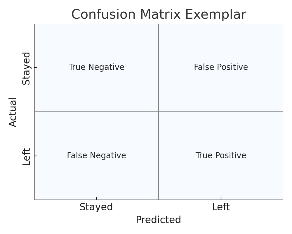
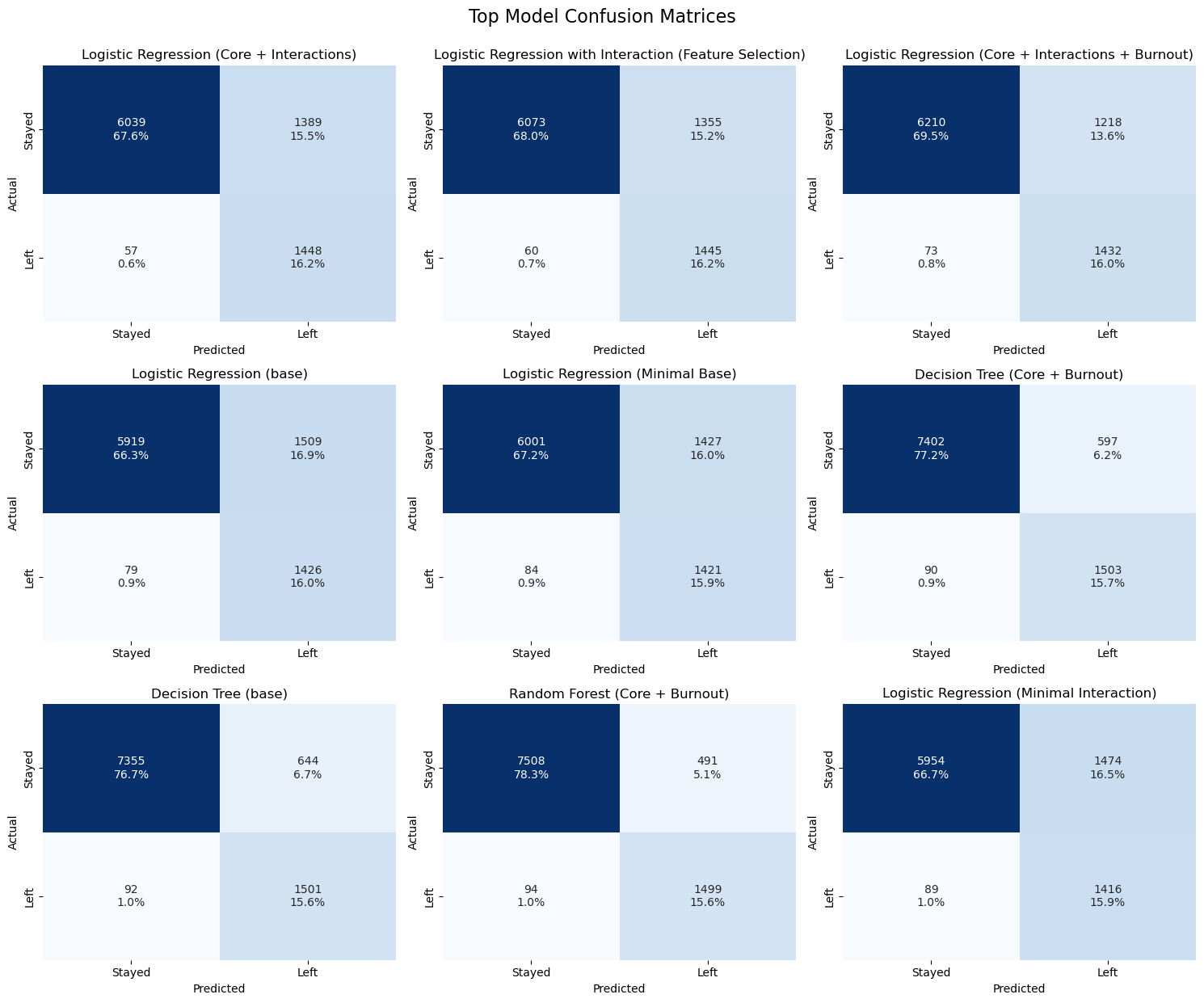
🔲 Confusion Matrix Results (All Selected Models, Training and Testing)¶

This section presents confusion matrices for each model on both training and holdout testing sets. The holdout test set represents 20% of the total dataset, while the training set represents 80%. Naturally, this results in lower absolute values in the second grid of confusion matrices. However, the relative percentages remain consistent, indicating well-calibrated model performance without signs of overfitting or underfitting.

Before:

After:

📋 Model Misclassification Summary¶

Model	Total Misclassified	False Positives (FP)	False Negatives (FN)
Logistic Regression	243	218	25
Decision Tree	149	127	22
Random Forest	145	123	22
XGBoost	79	55	24

Notes:

False Positives (FP): Predicted "Left", actually "Stayed"
False Negatives (FN): Predicted "Stayed", actually "Left"
Total Misclassified = FP + FN

Logistic Regression Interpretation¶

Back to top

Logistic Regression was evaluated as a baseline classifier to predict employee attrition. Despite its simplicity, it delivered strong performance in recall—correctly identifying approximately 93% of employees who left the company. This high sensitivity makes it valuable in contexts where catching potential churn is critical.

However, the model’s performance comes with trade-offs: notably, a higher false positive rate and signs of overconfidence in its predictions. Still, its interpretability and transparency offer meaningful insights into key attrition drivers, making it a useful diagnostic tool alongside more complex models.

Model	Recall	F2 Score	F1 Score	Precision	Accuracy	PR AUC	ROC AUC	Features	Confusion Matrix
Logistic Regression	0.933687	0.846968	0.743400	0.617544	0.891226	0.744055	0.948275	14	[[1639, 218], [25, 352]]

🔍 Feature Importance¶

Moderate workloads and satisfaction are protective. Longer tenure and higher average hours increase risk. Some binned features show effects opposite to their continuous versions due to multicollinearity. Non-linear effects are inherent to this prediciton task, exhibited in every model tested during development.

Strongest predictors of attrition (by absolute value):

projects_bin_medium (-2.14): Medium project load greatly reduces attrition risk.
tenure (+1.86): Longer tenure increases attrition risk.
hours_bin_medium (-1.47): Medium monthly hours reduce risk.
projects_bin_high (-1.26), hours_bin_high (-1.26): High project load or hours also reduce risk.
average_monthly_hours (+1.25): Higher average hours (continuous) increase risk.
satisfaction_level (-1.07): Higher satisfaction reduces risk.

Other effects:

satisfaction_bin_high (+0.79): High satisfaction (binned) increases risk (likely due to feature overlap).
tenure_bin_mid (-0.65): Mid-level tenure reduces risk.
number_project (+0.65): More projects (continuous) increase risk.
last_evaluation (+0.36): Higher evaluation slightly increases risk.
promotion_last_5years (-0.13): Recent promotion slightly reduces risk.
Other binned features: Small or negligible effects.

L1 regularization (Lasso) forced the logistic regression to ignore (zero out) or down-weight features that didn’t add much predictive value, especially in the presence of multicollinearity. This helps prevent overfitting and makes the model easier to interpret.

Feature	Coefficient
projects_bin_medium	-2.143055
tenure	1.860573
hours_bin_medium	-1.471872
projects_bin_high	-1.260723
hours_bin_high	-1.255469
average_monthly_hours	1.247562
satisfaction_level	-1.071616
satisfaction_bin_high	0.792443
tenure_bin_mid	-0.650269
number_project	0.646384
last_evaluation	0.357065
promotion_last_5years	-0.131051
satisfaction_bin_medium	0.048898
tenure_bin_long	0.000000

🔥SHAP summary plot¶

SHAP values (SHapley Additive exPlanations) provide detailed insight into how each feature influences individual predictions. Each dot represents an employee.

Color: Feature value (red = high, blue = low)
X-axis: Impact on prediction (negative = more likely to stay, positive = more likely to leave)

Key Insights:

High monthly hours (red) push predictions toward "Leave"—a classic sign of burnout. Conversely, low hours (blue) are associated with "Stay."
High satisfaction (red) strongly predicts "Stay," while very low satisfaction (blue) increases the likelihood of "Leave."
Longer tenure (red) is linked to "Leave" predictions, especially for employees with 2–5 years at the company (outliers >5 years were removed for logistic regression).
Number of projects shows a similar pattern: more projects shift predictions from "Stay" to "Leave."
Higher evaluations have a subtle effect, slightly increasing the chance of leaving.

Note: Ignore the binned features—multicollinearity limits interpretability for logistic regression in this context.

📉 Precision-Recall Curve¶

Shows the trade-off between precision and recall for different classification thresholds. It is especially useful for evaluating models on imbalanced datasets, as it focuses on the performance for the positive (minority) class.

The PR curve shows an immediate decline just under 0.8 precision, then levels off until about 0.8 recall, where it bends downwards fairly sharply. The model is strong at recall (few false negatives), but struggles with precision (a number of false positives). Average Precision (AP): 0.74

📋 Misclassification Analysis¶

The Logistic Regression model reflects classic class imbalance behavior:

False Positives (Actual = 0, Predicted = 1): The model frequently flagged employees as likely to leave when they actually stayed, and did so with high confidence (avg probability ~0.76). Many had low-to-moderate satisfaction, fairly high evaluations, and heavy workloads, suggesting it interpreted this as burnout and made confident predictions.
False Negatives (Actual = 1, Predicted = 0): The model struggled to detect a few employees who left despite being predicted to stay. These were generally low-risk profiles, with middling satisfaction, average workload, and no promotions. Predicted probabilities were very low (avg ~0.17), indicating the model wasn’t just wrong, it was confidently wrong.

In short, Logistic Regression is overconfident on both sides, but especially prone to confidently overpredicting attrition for burnout-like profiles.

🔴 False Positives (Predicted Left, Actually Stayed) — 218 cases¶

Feature	Mean	Std Dev	Min	Max
satisfaction_level	0.457	0.257	0.120	1.000
last_evaluation	0.722	0.172	0.360	1.000
number_project	3.71	1.57	2	6
average_monthly_hours	205.89	56.25	99	287
tenure	4.08	0.95	2	5
promotion_last_5years	0.005	0.068	0	1
predicted_proba	0.762	0.148	0.504	0.994

The model was highly confident these employees would leave, with many having probability > 0.9. But they stayed, likely due to organizational loyalty, resilience, or unmodeled factors like team culture or flexible hours. This misclassification points to a burnout signal the model leans too hard on.

🔵 False Negatives (Predicted Stay, Actually Left) — 25 cases¶

Feature	Mean	Std Dev	Min	Max
satisfaction_level	0.472	0.226	0.090	0.860
last_evaluation	0.709	0.173	0.450	1.000
number_project	4.08	1.32	2	7
average_monthly_hours	201.84	42.87	134	296
tenure	3.08	0.91	2	5
promotion_last_5years	0.000	0.000	0	0
predicted_proba	0.170	0.156	0.007	0.488

These low-confidence "stayers" left anyway. Their profiles didn’t raise red flags for the model: average satisfaction, moderate tenure, typical workload. Their attrition may be due to external personal factors or unobserved variables, such as lack of growth, poor management, or life events.

📊 Predicted Probability Distribution¶

The Logistic Regression model is notably overconfident, especially in its false positives:

When it incorrectly predicted "left" (actual = stayed), it often did so with very high confidence — a large cluster of predicted probabilities were above 0.9, and many more were spread throughout 0.5–0.9. The average proba was ~0.76, suggesting the model is certainly misclassifying some borderline loyal employees as churn risks.
When it incorrectly predicted "stayed" (actual = left), the predicted probabilities were consistently low, clustered below 0.1, with a small uptick near the decision threshold. The average proba was ~0.17.

This distribution indicates that the model is not well-calibrated: it's confident in its predictions — right or wrong — and less capable of expressing uncertainty. Logistic regression’s linearity and strong class imbalance likely contribute to this binary confidence profile.

🧠 Overall Assessment¶

While Logistic Regression falls short in precision compared to more advanced classifiers, its high recall and ease of interpretation justify its use as a baseline and explanatory model. It demonstrates a clear pattern: employees with medium workloads and satisfaction are at reduced risk, while longer tenure and high average hours are strong predictors of churn. Multicollinearity between binned and continuous features limits clean interpretability, but key patterns emerge nonetheless. Importantly, its misclassifications—especially confident false positives—highlight burnout-like profiles the model may overweigh. These findings can help shape feature engineering and interpret results from tree-based models that offer improved performance but reduced transparency.

Decision Tree Interpretation¶

Back to top

We evaluated a Decision Tree classifier to predict employee churn, using features related to employee engagement, performance, and demographics. The primary focus of this analysis was on recall, given the priority of identifying employees likely to leave. The model was relatively interpretable and performed reasonably well, though with evident trade-offs in precision and generalization.

Primary splits on satisfaction_level and tenure:
- Low satisfaction (≤0.47) and varying tenure/hours determine leave/stay decisions.
- Higher satisfaction (>0.47) combines with tenure and workload features.
Key decision nodes: low satisfaction + mid tenure + high hours = leave; high satisfaction + moderate workload = stay.

Model	Recall	F2 Score	F1 Score	Precision	Accuracy	PR AUC	ROC AUC	Features	Confusion Matrix
Decision Tree	0.944724	0.897375	0.834628	0.747515	0.937891	0.765587	0.956471	7	[[1874, 127], [22, 376]]

🌳 Decision Tree Summary¶

🌟 Primary Split:¶

satisfaction_level ≤ 0.47 → More likely to Leave, especially with low tenure or high hours.
satisfaction_level > 0.47 → More likely to Stay, especially if tenure is low and projects/hours are moderate.

🟥 If satisfaction_level ≤ 0.47:¶

📌 Tenure ≤ 4.5¶

Tenure ≤ 2.5
- Very low satisfaction (≤ 0.15) and moderate-to-high hours → Left
- Else → Stayed
Tenure > 2.5
- Low hours or low evaluation → Stayed
- High evaluation → Left

📌 Tenure > 4.5¶

Very low satisfaction (≤ 0.11) → Left
Else:
- Many projects or very high hours → Left
- Fewer projects and moderate hours → Stayed

✅ If satisfaction_level > 0.47:¶

📌 Tenure ≤ 4.5¶

Hours ≤ 290.5
- Projects ≤ 6 → Stayed
- Projects > 6 → Left
Hours > 290.5 → Left, regardless of satisfaction level (even if > 0.63)

📌 Tenure > 4.5¶

Last eval ≤ 0.81
- Projects ≤ 6 → Stayed
- Projects > 6 → Left
Last eval > 0.81
- Low hours → Stayed
- High hours → Left, unless tenure is very high (> 6.5)

🔑 Key Features Driving Decisions:¶

satisfaction_level
tenure
average_monthly_hours
number_project
last_evaluation

🌳 Scrollable Outline with Splits:¶

🌳 |--- satisfaction_level <= 0.47
🌳 |   |--- tenure <= 4.50
🌳 |   |   |--- tenure <= 2.50
🌳 |   |   |   |--- satisfaction_level <= 0.15
🌳 |   |   |   |   |--- average_monthly_hours <= 129.00
🍃 |   |   |   |   |   |--- class: Stayed | Value = [Stayed: 1, Left: 0]
🌳 |   |   |   |   |--- average_monthly_hours >  129.00
🍃 |   |   |   |   |   |--- class: Stayed | Value = [Stayed: 107, Left: 15]
🌳 |   |   |   |--- satisfaction_level >  0.15
🌳 |   |   |   |   |--- average_monthly_hours <= 247.00
🍃 |   |   |   |   |   |--- class: Left | Value = [Stayed: 330, Left: 3097]
🌳 |   |   |   |   |--- average_monthly_hours >  247.00
🍃 |   |   |   |   |   |--- class: Left | Value = [Stayed: 282, Left: 3097]
🌳 |   |   |--- tenure >  2.50
🌳 |   |   |   |--- average_monthly_hours <= 125.50
🍃 |   |   |   |   |--- class: Stayed | Value = [Stayed: 262, Left: 195]
🌳 |   |   |   |--- average_monthly_hours >  125.50
🌳 |   |   |   |   |--- last_evaluation <= 0.44
🍃 |   |   |   |   |   |--- class: Stayed | Value = [Stayed: 262, Left: 54]
🌳 |   |   |   |   |--- last_evaluation >  0.44
🍃 |   |   |   |   |   |--- class: Left | Value = [Stayed: 14, Left: 21]
🌳 |   |--- tenure >  4.50
🌳 |   |   |--- satisfaction_level <= 0.11
🍃 |   |   |   |--- class: Stayed | Value = [Stayed: 3727, Left: 177]
🌳 |   |   |--- satisfaction_level >  0.11
🌳 |   |   |   |--- number_project <= 6.50
🌳 |   |   |   |   |--- average_monthly_hours <= 276.50
🍃 |   |   |   |   |   |--- class: Stayed | Value = [Stayed: 552, Left: 60]
🌳 |   |   |   |   |--- average_monthly_hours >  276.50
🍃 |   |   |   |   |   |--- class: Stayed | Value = [Stayed: 60, Left: 24]
🌳 |   |   |   |--- number_project >  6.50
🍃 |   |   |   |   |--- class: Left | Value = [Stayed: 0, Left: 12]
🌳 |--- satisfaction_level >  0.47
🌳 |   |--- tenure <= 4.50
🌳 |   |   |--- average_monthly_hours <= 290.50
🌳 |   |   |   |--- number_project <= 5.50
🌳 |   |   |   |   |--- tenure <= 3.50
🍃 |   |   |   |   |   |--- class: Stayed | Value = [Stayed: 174, Left: 30]
🌳 |   |   |   |   |--- tenure >  3.50
🍃 |   |   |   |   |   |--- class: Left | Value = [Stayed: 0, Left: 3]
🌳 |   |   |   |--- number_project >  5.50
🌳 |   |   |   |   |--- number_project <= 6.50
🍃 |   |   |   |   |   |--- class: Stayed | Value = [Stayed: 24, Left: 24]
🌳 |   |   |   |   |--- number_project >  6.50
🍃 |   |   |   |   |   |--- class: Left | Value = [Stayed: 47, Left: 1237]
🌳 |   |   |--- average_monthly_hours >  290.50
🌳 |   |   |   |--- satisfaction_level <= 0.63
🍃 |   |   |   |   |--- class: 
🌳 |   |   |   |--- satisfaction_level >  0.63
🍃 |   |   |   |   |--- class: 
🌳 |   |--- tenure >  4.50
🌳 |   |   |--- last_evaluation <= 0.81
🌳 |   |   |   |--- number_project <= 6.50
🌳 |   |   |   |   |--- tenure <= 6.50
🍃 |   |   |   |   |   |--- class: 
🌳 |   |   |   |   |--- tenure >  6.50
🍃 |   |   |   |   |   |--- class: 
🌳 |   |   |   |--- number_project >  6.50
🍃 |   |   |   |   |--- class: 
🌳 |   |   |--- last_evaluation >  0.81
🌳 |   |   |   |--- average_monthly_hours <= 216.50
🌳 |   |   |   |   |--- tenure <= 5.50
🍃 |   |   |   |   |   |--- class: 
🌳 |   |   |   |   |--- tenure >  5.50
🍃 |   |   |   |   |   |--- class: 
🌳 |   |   |   |--- average_monthly_hours >  216.50
🌳 |   |   |   |   |--- tenure <= 6.50
🍃 |   |   |   |   |   |--- class: 
🌳 |   |   |   |   |--- tenure >  6.50
🍃 |   |   |   |   |   |--- class: 

🔍 Feature Importance¶

The tree overwhelmingly relies on tenure and satisfaction_level, which jointly make up over 84% of the total feature importance. These are highly intuitive predictors for churn, where low satisfaction or mid-length tenure employees are at higher risk.

Feature	Importance
tenure	0.421398
satisfaction_level	0.420542
last_evaluation	0.092148
average_monthly_hours	0.054863
number_project	0.011049
promotion_last_5years	0.000000
burnout	0.000000

📉 Precision-Recall Curve¶

Shows the trade-off between precision and recall for different classification thresholds. It is especially useful for evaluating models on imbalanced datasets, as it focuses on the performance for the positive (minority) class.

The PR curve shows a gentle decline in precision from 1.0 to ~0.825, gradually leveling off around 0.2 recall, falling sharply past 0.95 recall. The model is strong at recall (few false negatives), but not perfect at precision (some false positives). Average Precision (AP): 0.77

📋 Misclassification Analysis¶

False predictions cluster mostly around 3–4 years of tenure and low satisfaction, confirming our expectations from the feature importance rankings.

🔴 False Positives (Predicted Left, Actually Stayed) — 127 cases¶

Feature	Mean	Std Dev	Min	Max
Satisfaction Level	0.313	0.171	0.12	0.90
Last Evaluation	0.750	0.155	0.45	1.00
Number of Projects	4.23	1.31	2	6
Monthly Hours	213.19	46.76	126	287
Tenure (Years)	3.87	0.86	3	6
Promotion (5 Years)	1.57%	12.50%	0.0%	100.0%
Predicted Probability	0.910	0.086	0.584	0.975

False positives overwhelmingly had low satisfaction, average evaluation scores, and clustered around 3–4 years of tenure, a tenure range linked to higher voluntary turnover but here misjudged.

🔵 False Negatives (Predicted Stay, Actually Left) — 22 cases¶

Feature	Mean	Std Dev	Min	Max
Satisfaction Level	0.636	0.189	0.17	0.89
Last Evaluation	0.700	0.143	0.45	1.00
Number of Projects	4.18	1.05	2	6
Monthly Hours	213.95	52.59	128	281
Tenure (Years)	3.64	1.47	2	6
Promotion (5 Years)	0.0%	0.0%	0.0%	0.0%
Predicted Probability	0.095	0.079	0.024	0.285

False negatives had moderate satisfaction, but still within the dissatisfaction spectrum (relative to leavers). These are likely borderline churn risks, not flagged confidently enough by the tree.

📊 Predicted Probability Distribution¶

The predicted probabilities for misclassified cases reveal a strong overconfidence by the Decision Tree model:

When the model incorrectly predicted "left" (actual = stayed), it was highly confident, with probabilities clustered around 0.91 (mean = 0.91, min = 0.58, max = 0.97).
When the model incorrectly predicted "stayed" (actual = left), it was again quite confident, with probabilities averaging 0.095 (min = 0.02, max = 0.28).

This indicates that while the model performs well overall, its errors are made with high confidence, lacking probabilistic nuance. In contrast to more calibrated classifiers like Random Forest or Logistic Regression, the Decision Tree makes binary, decisive predictions even when wrong.

🧠 Overall Assessment¶

The Decision Tree model captures key churn drivers well, especially satisfaction level and tenure, and demonstrates decent recall performance. However, it suffers from a binary confidence pattern and occasional overreach, especially in employees that fit the pattern of high-risk of departure, at 3–4 year tenure with low satisfaction, leading to a number of false positives.

Future model improvement could include pruning or ensemble methods (e.g., Random Forest, XGBoost - see below) to smooth out prediction certainty and reduce overfitting around hard splits. For operational use, threshold tuning and targeted interventions on mid-tenure, low-satisfaction employees may prove most effective.

Random Forest Interpretation¶

Back to top

The Random Forest model performed slightly better than the Decision Tree, maintaining a strong recall (0.945) and improving marginally in precision and F₂ score. It strikes a reliable balance between catching most leavers and minimizing false positives. However, like most ensemble models, interpretability is reduced compared to single-tree models. Feature importance is heavily skewed toward satisfaction level and tenure, which dominate model decisions.

Model	Recall	F2 Score	F1 Score	Precision	Accuracy	PR AUC	ROC AUC	Features	Confusion Matrix
Random Forest	0.944724	0.899091	0.838350	0.753507	0.939558	0.946198	0.978260	7	[[1878, 123], [22, 376]]

🔍 Feature Importance¶

The tree overwhelmingly relies on satisfaction_level and tenure, which jointly make up over 83% of the total feature importance. These are highly intuitive predictors for churn, where low satisfaction or mid-length tenure employees are at higher risk.

Feature	Importance
satisfaction_level	0.420294
tenure	0.411007
last_evaluation	0.095843
average_monthly_hours	0.054253
number_project	0.018581
burnout	0.000012
promotion_last_5years	0.000010

📉 Precision-Recall Curve¶

Shows the trade-off between precision and recall for different classification thresholds. It is especially useful for evaluating models on imbalanced datasets, as it focuses on the performance for the positive (minority) class.

The PR curve is nearly linear and hovers close to 1.0, sharply declining only at very high recall values, reflecting the model’s stability in identifying true positives.
Average Precision (AP): 0.95

📋 Misclassification Analysis¶

The Random Forest model showed similar patterns to XGBoost in terms of error type and confidence levels:

False Positives (Actual = 0, Predicted = 1): Most had low satisfaction but high evaluation, with a high predicted probability (avg ~0.82). The model was very confident they would leave.
False Negatives (Actual = 1, Predicted = 0): These were employees with moderate-to-high satisfaction, but predicted to stay with low confidence (avg proba ~0.13), again suggesting strong class separation.

It's exhibiting model behavior typical of class imbalance with high separability for only one class (burned-out leavers). It’s doing a decent job overall, but it keeps misclassifying those edge-case stayers (burned-out but loyal) and quiet quitters (who look fine but leave).

🔴 False Positives (Predicted Left, Actually Stayed) — 123 cases¶

Feature	Mean	Std Dev	Min	Max
satisfaction_level	0.316	0.173	0.120	0.900
last_evaluation	0.751	0.152	0.450	1.000
number_project	4.20	1.32	2	6
average_monthly_hours	210.98	45.83	126	287
tenure	3.82	0.83	3	6
promotion_last_5years	0.02	0.13	0	1
predicted_proba	0.8220	0.0634	0.5046	0.9772

Most false positives had very high model confidence, with probabilities consistently >0.5. Indicates overconfidence in identifying at-risk employees with medium dissatisfaction.

Strong confidence these people were going to leave (but they didn’t).
These false positives are driven by low satisfaction_level (mean = 0.316).
Many had high last_evaluation, high monthly_hours, and a decent number of projects (median = 5).
Burnout signal again.

🔵 False Negatives (Predicted Stay, Actually Left) — 22 cases¶

Feature	Mean	Std Dev	Min	Max
satisfaction_level	0.636	0.189	0.170	0.890
last_evaluation	0.700	0.143	0.450	1.000
number_project	4.18	1.05	2	6
average_monthly_hours	213.95	52.59	128	281
tenure	3.64	1.47	2	6
promotion_last_5years	0.00	0.00	0	0
predicted_proba	0.1262	0.1228	0.0265	0.4287

False negatives were low-confidence predictions, indicating the model generally "believed" they would stay, but without high certainty. Indicates model confusion when people seem reasonably content but still exit, perhaps due to personal reasons not captured in data.

Low confidence they were going to stay (and they didn't stay).
These are false negatives.
These employees had decent satisfaction (mean = 0.636), decent evaluations, average monthly hours (~214), and again, no promotions, low tenure (median = 3.5), and almost all not flagged as burned out.
These are probably low-risk leavers the model doesn't know how to spot well.

📊 Predicted Probability Distribution¶

The predicted probabilities for misclassified cases show that the Random Forest model, while better calibrated than the Decision Tree, still makes confident errors:

When the model incorrectly predicted "left" (actual = stayed), it was fairly confident, with probabilities clustered around 0.82 (min = 0.50, max = 0.98).
When the model incorrectly predicted "stayed" (actual = left), it showed low predicted probabilities, averaging 0.13 (min = 0.03, max = 0.43).

This suggests the model is more probabilistically nuanced than the Decision Tree, but it still tends to overcommit on burned-out-looking employees leaving, and struggles to catch a few lower-risk leavers.

🧠 Overall Assessment¶

The Random Forest model balances recall and precision well, with improved calibration over a single tree. The model, like most classifiers in this context, struggles with "gray area" employees who fall between clear satisfaction and dissatisfaction thresholds. This is expected in real-world HR analytics, where exits often happen for unmeasurable or personal reasons (e.g., career growth, relocation, family needs, interpersonal conflict, or random opportunity). This intrinsic uncertainty places a ceiling on prediction accuracy, especially when limited features are available.

XGBoost Interpretation¶

Back to top

XGBoost performed exceptionally well across all evaluation metrics, demonstrating high precision and recall, as well as excellent overall accuracy.

Model	Recall	F2 Score	F1 Score	Precision	Accuracy	PR AUC	ROC AUC	Features	Confusion Matrix
XGBoost	0.939698	0.925285	0.904474	0.871795	0.967070	0.966941	0.982202	7	[[1946, 55], [24, 374]]

🔍 Feature Importance¶

The tree overwhelmingly relies on satisfaction_level and tenure, which jointly make up over 83% of the total feature importance. These are highly intuitive predictors for churn, where low satisfaction or mid-length tenure employees are at higher risk.

Feature	Importance
satisfaction_level	0.420294
tenure	0.411007
last_evaluation	0.095843
average_monthly_hours	0.054253
number_project	0.018581
burnout	0.000012
promotion_last_5years	0.000010

🔥SHAP summary plot¶

SHAP values (SHapley Additive exPlanations) provide detailed insight into how each feature influences individual predictions. Each dot represents an employee.

Color: Feature value (red = high, blue = low)
X-axis: Impact on prediction (negative = more likely to stay, positive = more likely to leave)

Key Insights:

High satisfaction (red) strongly predicts “Stay.”
Very low satisfaction (blue) increases the likelihood of “Leave.”
High tenure (red) is linked to “Leave” predictions, but very high tenure swings back toward “Stay” (as seen in EDA). Low tenure generally predicts “Stay.”
Low project count (blue) (disengaged) and very high project count (red) (burnout) both increase risk of leaving.
Very high hours (red) are associated with leaving; low hours (blue) with staying. The middle range is mixed, with a slight lean toward staying.
High evaluations (red) slightly push toward leaving, while many lower-evaluated employees (blue) stay, suggesting some high performers are at risk.

📉 Precision-Recall Curve¶

Shows the trade-off between precision and recall for different classification thresholds. It is especially useful for evaluating models on imbalanced datasets, as it focuses on the performance for the positive (minority) class.

The PR curve is nearly linear and hovers close to 1.0, sharply declining only at very high recall values, reflecting the model’s stability in identifying true positives.
Average Precision (AP): 0.97

📋 Misclassification Analysis¶

Misclassified examples are broadly distributed across different levels of tenure and satisfaction. Some false positives (predicted leave, actually stayed) cluster around satisfaction levels of 0.35 and 0.85, but counts remain in single digits.

🔴 False Positives (Predicted Left, Actually Stayed) — 55 cases¶

Feature	Mean	Std Dev	Min	Max
satisfaction_level	0.581	0.217	0.130	0.900
last_evaluation	0.749	0.185	0.450	1.000
number_project	3.84	1.50	2	6
average_monthly_hours	210.27	56.94	126	286
tenure	4.58	0.98	2	6
promotion_last_5years	0.02	0.13	0	1
predicted_proba	0.7425	0.1403	0.5016	0.9826

Most false positives had moderately high confidence.

🔵 False Negatives (Predicted Stay, Actually Left) — 24 cases¶

Feature	Mean	Std Dev	Min	Max
satisfaction_level	0.555	0.229	0.170	0.890
last_evaluation	0.663	0.134	0.450	0.990
number_project	4.17	1.05	2	6
average_monthly_hours	212.67	47.61	128	281
tenure	3.58	1.28	2	6
promotion_last_5years	0.00	0.00	0	0
predicted_proba	0.1190	0.1022	0.0088	0.3481

False negatives generally had low predicted probabilities, suggesting the model was confident they would stay.

📊 Predicted Probability Distribution¶

The XGBoost model shows more spread and nuance in its misclassified predictions than the Decision Tree or Random Forest, but still leans toward overconfidence:

When it incorrectly predicted "left" (actual = stayed), predicted probabilities were high but more varied, with a mean of 0.74 and a range from 0.50 to 0.98.
When it incorrectly predicted "stayed" (actual = left), it tended to be underconfident, with probabilities centered around 0.12 (min = 0.01, max = 0.35).

This distribution suggests that XGBoost, while not perfectly calibrated, preserves more probabilistic uncertainty, especially compared to the binary overconfidence of the Decision Tree. It's more cautious — but still misses on both sides.

🧠 Overall Assessment¶

XGBoost outperformed all other models on nearly every metric. It balances strong discrimination and improved calibration over simpler models. Its high recall, precision, and AUC make it a strong candidate for deployment, particularly when correctly identifying leavers is critical. The tree overwhelmingly relies on tenure and satisfaction level to make predictions. Misclassification patterns reinforce the idea that the model struggles most with borderline cases, employees with mid-to-low satisfaction around years 3–4. These are often ambiguous profiles: employees possibly dissatisfied but not clearly on the way out.

Overall, XGBoost provides the strongest predictive performance of all models tested. However, its complexity and opacity may present interpretability challenges in an HR context, especially for stakeholders who require transparent decision logic.

Cross‑Model Reflection¶

Back to top

XGBoost shows the strongest predictive performance.
All models consistently show turnover related to extreme workloads and around 4 years of tenure.
All models show difficulty with borderline “gray‑area” employees (mid tenure with moderate dissatisfaction), highlighting challenges inherent in HR predictive modeling.
This reflects real-world turnover motivations (e.g., opportunities, life changes) not captured by features, an expected limitation of the model.
To improve edge‑case predictions: consider incorporating more behavioral or temporal features, employing probability calibration, or using mixed-methods (e.g., qualitative feedback) alongside these models.

Conclusion¶

Back to top

This section presents a concluding summary of model strengths with key insights for business decision-making.

Narrative Summary & Business Insights¶

The predictive models developed for employee attrition at Salifort Motors consistently identified key risk factors such as low satisfaction, high workload, and mid-level tenure. They also revealed a persistent challenge: all models struggled to accurately predict outcomes for “gray-area” employees, particularly those with moderate dissatisfaction and 3-4 years of tenure. This limitation reflects the complex, multifaceted nature of turnover, where personal motivations and external factors often go unmeasured.

Key Business Insights:¶

Burnout and Disengagement: Employees with low satisfaction or extreme workloads (high and low) are at highest risk. Monitoring these factors, especially for those at the 3-4 year mar, should be a priority.
Borderline Cases: Many misclassifications occurred among employees who did not fit clear risk profiles, highlighting the need for richer data (e.g., behavioral signals, qualitative feedback) and more nuanced modeling.
Retention Levers: Opportunities for advancement, recognition, and work-life balance emerged as actionable levers to reduce attrition risk.
Model as Early Warning: The model is best used as an early warning system to flag at-risk employees for supportive HR outreach, not as a punitive tool.

Actionable Strategies:¶

To reduce churn, Salifort Motors should prioritize monitoring, enhance communication and culture, provide proactive support, implement effective workload policies, and strengthen recognition and retention programs.

Monitor Satisfaction & Workload: Conduct regular employee satisfaction surveys and track workload metrics to identify early signs of burnout or disengagement.
Communicate Predictive Modeling Transparently: Explain how employee prediction models are used, reinforcing a message of fairness, support, and shared accountability.
Discuss Company Culture Openly: Facilitate regular, inclusive discussions about company culture-its values, expectations, and how it’s experienced by employees.
Clarify Workload Expectations: Define standard workload ranges and communicate overtime policies transparently, including compensation structures where applicable.
Set Limits on Projects and Hours: Implement clear caps on project assignments and monthly hours to reduce burnout and promote sustainable productivity.
Support Work-Life Balance: Encourage healthy workloads and reasonable scheduling to foster long-term employee wellbeing.
Conduct Stay Interviews: Schedule proactive conversations with employees nearing critical tenure milestones (e.g., year 4) to surface concerns before they become resignations.
Advance and Recognize Talent: Increase promotion and recognition opportunities, particularly around the 4-year mark, to reinforce engagement and retention.
Targeted Retention Strategies: Prioritize support for employees with low satisfaction and extreme workloads, especially those in the 3–4 year tenure window, where churn risk peaks.

Next Steps:¶

Model Deployment: Integrate the model into HR processes for early identification of at-risk employees.
Continuous Improvement: Retrain and calibrate the model as new data becomes available; expand data sources to include engagement surveys and qualitative feedback.
Bias & Fairness Audits: Routinely check for bias and monitor for unintended consequences.
Ethical Safeguards: Ensure employee data privacy, fairness, and transparency in all predictive analytics initiatives.

Ethical Considerations:¶

Maintain strict data privacy. Use predictions to support, not penalize, employees. Communicate transparently about the model’s purpose and limitations. Regular audits for bias and fairness are essential to uphold trust and integrity.

In summary, while predictive modeling offers valuable guidance for HR strategy, its greatest value lies in augmenting, not replacing, human judgment and supportive engagement. Combining model insights with ongoing feedback and ethical safeguards will help Salifort Motors proactively retain talent and foster a healthier workplace.

Continue Exploring:

Executive Summary

Exploratory Data Analysis

Appendix: Data Dictionary¶

Back to top

Original Dataset¶

After removing duplicates, the dataset contained 11,991 rows and 10 columns for the variables listed below.

Note: For more information about the data, refer to its source on Kaggle.

Variable	Description
satisfaction_level	Employee-reported job satisfaction level [0–1]
last_evaluation	Score of employee's last performance review [0–1]
number_project	Number of projects employee contributes to
average_monthly_hours	Average number of hours employee worked per month
time_spend_company	How long the employee has been with the company (years)
Work_accident	Whether or not the employee experienced an accident while at work
left	Whether or not the employee left the company
promotion_last_5years	Whether or not the employee was promoted in the last 5 years
Department	The employee's department
salary	The employee's salary (U.S. dollars)

Feature Engineering Data Dictionary¶

The following table describes the engineered features created for model development. These features are derived from the original dataset using binning, interaction terms, and logical flags to capture important patterns identified during exploratory data analysis.

Variable	Description
Bins
satisfaction_bin_low	Binary indicator: satisfaction_level is low (≤ 0.4)
satisfaction_bin_medium	Binary indicator: satisfaction_level is medium (> 0.4 and ≤ 0.7)
satisfaction_bin_high	Binary indicator: satisfaction_level is high (> 0.7)
hours_bin_low	Binary indicator: average_monthly_hours is low (≤ 160)
hours_bin_medium	Binary indicator: average_monthly_hours is medium (> 160 and ≤ 240)
hours_bin_high	Binary indicator: average_monthly_hours is high (> 240)
projects_bin_low	Binary indicator: number_project is low (≤ 2)
projects_bin_medium	Binary indicator: number_project is medium (> 2 and ≤ 5)
projects_bin_high	Binary indicator: number_project is high (> 5)
tenure_bin_short	Binary indicator: tenure is short (≤ 3 years)
tenure_bin_mid	Binary indicator: tenure is mid (> 3 and ≤ 5 years)
tenure_bin_long	Binary indicator: tenure is long (> 5 years)
Interactions
satisfaction_x_projects	Interaction: satisfaction_level × number_project
satisfaction_x_hours	Interaction: satisfaction_level × average_monthly_hours
evaluation_x_satisfaction	Interaction: last_evaluation × satisfaction_level
hours_per_project	Ratio: average_monthly_hours divided by number_project
Flags
burnout	Flag: True if (number_project ≥ 6 or average_monthly_hours ≥ 240) and satisfaction_level ≤ 0.3
disengaged	Flag: True if (number_project ≤ 2 and average_monthly_hours < 160 and satisfaction_level ≤ 0.5)
no_promo_4yr	Flag: True if promotion_last_5years == 0 and tenure ≥ 4

Note:
Binned features are one-hot encoded as separate columns (e.g., satisfaction_bin_low, satisfaction_bin_medium, satisfaction_bin_high). Only the relevant dummy variables (excluding the first category for each bin) are included in the final dataset, depending on the encoding strategy.

Appendix: Feature Engineering¶

Back to Top

In addition to baseline models run with all original features, all feature engineering varieties below were tested with all four model types: Logistic Regression, Decision Tree, Random Forest, and XGBoost.

Feature Engineering Round One¶

Original features + binning: This set adds binned versions of key variables (satisfaction, workload, projects, tenure) to the original features. Binning helps capture non-linear effects and threshold-based risk groups identified in EDA (e.g., low/medium/high satisfaction, extreme workloads, tenure windows).

Original features + interactions: This set augments the original features with interaction terms that capture relationships between satisfaction, workload, and performance (e.g., satisfaction × projects, satisfaction × hours, evaluation × satisfaction, hours per project). These interactions help distinguish between disengaged, overworked, and healthy employees.

Original features + categorical flags: This set adds logical flag features to the original data, such as "burnout" (overworked and dissatisfied), "disengaged" (underworked and dissatisfied), and "no_promo_4yr" (long tenure without promotion). These flags directly encode high-risk employee profiles identified in EDA.

Feature selection: For each of the above, a feature selection variant was also run, dropping weak predictors (department, salary, work_accident) to reduce noise and multicollinearity, especially for logistic regression.

Feature Engineering Round Two¶

Selected features + burnout flag: This set isolates the core predictors of attrition (satisfaction, workload, tenure, promotion) and adds a “burnout” flag to capture the high-risk group of overworked, dissatisfied employees

Selected features + interactions: This set focuses on the main drivers (satisfaction, workload, tenure) and adds interaction terms (satisfaction × projects, hours per project) to capture non-linear effects and workload intensity, which EDA showed are important for distinguishing between underworked, overworked, and healthy employees.

Selected features + interactions + burnout flag: This feature set combines the core predictors of attrition (satisfaction, workload, tenure) with a “burnout” flag to capture high-risk, overworked employees. It also includes a key interaction term, "satisfaction × projects", to distinguish between groups identified in EDA

Appendix: Hyperparameter Tuning Grids¶

Back to Top

This section summarizes the hyperparameter grids used for model selection and tuning via GridSearchCV and RandomizedSearchCV for all baseline and feature-engineered models.

Logistic Regression¶

Baseline Grid:

lr_base_param_grid = {
    "Logistic Regression": {
        "model__C": [0.01, 0.1, 1.0, 10.0, 100.0],  # Regularization strength (inverse)
        "model__penalty": ["l1", "l2"],             # L1 (Lasso) or L2 (Ridge)
        "model__solver": ["liblinear"],             # Supports L1/L2
        "model__class_weight": [None, "balanced"],  # Handle class imbalance
    }
}

Feature Engineering Grid:

lr_fe_params = {
    "model__C": [0.1, 1.0, 10.0],
    "model__penalty": ["l1", "l2"],
    "model__solver": ["liblinear"],
    "model__class_weight": [None, "balanced"],
}

Decision Tree¶

Baseline Grid:

tree_base_param_grids = {
    "Decision Tree": {
        "model__max_depth": [4, 6, 8, None],        # Max tree depth
        "model__min_samples_leaf": [1, 2, 5],       # Min samples at leaf
        "model__min_samples_split": [2, 4, 6],      # Min samples to split
        "model__class_weight": [None, "balanced"],  # Handle class imbalance
    },
    ...
}

Feature Engineering Grid:

tree_fe_params = {
    "Decision Tree": {
        "model__max_depth": [3, 4, 5, 6, 8],
        "model__min_samples_leaf": [1, 2, 3],
        "model__min_samples_split": [2, 3, 4],
        "model__class_weight": [None, "balanced"],
    },
    ...
}

Random Forest¶

Baseline Grid:

tree_base_param_grids = {
    "Random Forest": {
        "model__n_estimators": [300, 500],          # Number of trees
        "model__max_depth": [3, 5, None],           # Max tree depth
        "model__max_features": ["sqrt", 1.0],       # Features considered at each split
        "model__max_samples": [0.7, 1.0],           # Fraction of samples per tree
        "model__min_samples_leaf": [1, 2, 3],       # Min samples at leaf
        "model__min_samples_split": [2, 3, 4],      # Min samples to split
        "model__class_weight": [None, "balanced"],  # Handle class imbalance
    },
    ...
}

Feature Engineering Grid:

tree_fe_params = {
    "Random Forest": {
        "model__n_estimators": [100, 300],
        "model__max_depth": [3, 4, 5, 8],
        "model__max_features": ["sqrt", 1.0],
        "model__max_samples": [0.7, 1.0],
        "model__min_samples_leaf": [1, 2],
        "model__min_samples_split": [2, 3],
        "model__class_weight": [None, "balanced"],
    },
    ...
}

XGBoost¶

Baseline Grid:

tree_base_param_grids = {
    "XGBoost": {
        "model__n_estimators": [100, 300],              # Number of boosting rounds
        "model__max_depth": [3, 5, 7],                  # Max tree depth
        "model__learning_rate": [0.01, 0.1, 0.2],       # Step size shrinkage
        "model__subsample": [0.6, 0.8, 1.0],            # Row subsampling
        "model__colsample_bytree": [0.6, 0.8, 1.0],     # Feature subsampling
        "model__min_child_weight": [1, 5, 10],          # Min sum of instance weight in a child
        "model__gamma": [0, 0.1, 0.2],                  # Min loss reduction to split
        "model__scale_pos_weight": [1, scale_pos_weight_value],  # Class imbalance
    },
    ...
}

Feature Engineering Grid:

tree_fe_params = {
    "XGBoost": {
        "model__n_estimators": [100, 300],
        "model__max_depth": [3, 4, 5, 8],
        "model__learning_rate": [0.1, 0.2],
        "model__subsample": [0.6, 0.8, 1.0],
        "model__colsample_bytree": [0.6, 0.8, 1.0],
        "model__min_child_weight": [1, 5],
        "model__gamma": [0, 0.1, 0.2],
        "model__scale_pos_weight": [1, scale_pos_weight_value],
        "model__reg_alpha": [0, 0.1, 1],            # L1 regularization
        "model__reg_lambda": [1, 2, 5],             # L2 regularization
    },
    ...
}

Notes:

All hyperparameters were tuned using either GridSearchCV (for smaller grids or faster models) or RandomizedSearchCV (for larger grids or slower models).
scale_pos_weight_value is dynamically calculated as the ratio of negative to positive samples in the training set to address class imbalance for XGBoost.
For all models, model__class_weight="balanced" was included as an option to help mitigate class imbalance.
Feature engineering grids used slightly smaller or more regularized search spaces for efficiency.

Model Construction and Validation

Predicting employee turnover at Salifort Motors¶

Table of Contents¶

Description and Deliverables¶

This page summarizes the second part of the project: predictive model construction and validation, with interpretation of results.¶

Exploratory Data Analysis Insights¶

A quick recap of the exploratory data analysis:¶

Modeling Strategies Recap¶

Approach¶

Lessons Learned¶

Final Model Selection¶

Next Steps¶

Cross-Validation Results¶

Model Selection¶

Model Evaluation Strategy¶

Tie-Breaker Criteria for Model Selection¶

Logistic Regression Selection¶

Data Dictionary:¶

Decision Tree Selection¶

Data Dictionary:¶

Random Forest Selection¶

Data Dictionary:¶

XGBoost Selection¶

Data Dictionary:¶

Model Results & Interpretation¶

📝 Model Evaluation Summary¶

🧠 Technical Model Performance Summary¶

🔲 Confusion Matrix Results (All Selected Models, Training and Testing)¶

📋 Model Misclassification Summary¶

Logistic Regression Interpretation¶

🔍 Feature Importance¶

🔥SHAP summary plot¶

📉 Precision-Recall Curve¶

📋 Misclassification Analysis¶

🔴 False Positives (Predicted Left, Actually Stayed) — 218 cases¶

🔵 False Negatives (Predicted Stay, Actually Left) — 25 cases¶

📊 Predicted Probability Distribution¶

🧠 Overall Assessment¶

Decision Tree Interpretation¶

🌳 Decision Tree Summary¶

🌟 Primary Split:¶

🟥 If satisfaction_level ≤ 0.47:¶

📌 Tenure ≤ 4.5¶

📌 Tenure > 4.5¶

✅ If satisfaction_level > 0.47:¶

📌 Tenure ≤ 4.5¶

📌 Tenure > 4.5¶

🔑 Key Features Driving Decisions:¶

🌳 Scrollable Outline with Splits:¶

🔍 Feature Importance¶

📉 Precision-Recall Curve¶

📋 Misclassification Analysis¶

🔴 False Positives (Predicted Left, Actually Stayed) — 127 cases¶

🔵 False Negatives (Predicted Stay, Actually Left) — 22 cases¶

📊 Predicted Probability Distribution¶

🧠 Overall Assessment¶

Random Forest Interpretation¶

🔍 Feature Importance¶

📉 Precision-Recall Curve¶

📋 Misclassification Analysis¶

🔴 False Positives (Predicted Left, Actually Stayed) — 123 cases¶

🔵 False Negatives (Predicted Stay, Actually Left) — 22 cases¶

📊 Predicted Probability Distribution¶

🧠 Overall Assessment¶

XGBoost Interpretation¶

🔍 Feature Importance¶

🔥SHAP summary plot¶

📉 Precision-Recall Curve¶

📋 Misclassification Analysis¶

🔴 False Positives (Predicted Left, Actually Stayed) — 55 cases¶

🔵 False Negatives (Predicted Stay, Actually Left) — 24 cases¶

📊 Predicted Probability Distribution¶

🧠 Overall Assessment¶

Cross‑Model Reflection¶

Conclusion¶

Narrative Summary & Business Insights¶

Key Business Insights:¶

Actionable Strategies:¶

Next Steps:¶

Ethical Considerations:¶