
Executive Summary
Understanding and predicting employee turnover at Salifort Motors
Bryan Johns
June 2025
Note:
Completed as the capstone for the Google Advanced Data Analytics Certificate, in true autodidact fashion I took this project as the opportunity to go far beyond the minimum requirements and really explore the ins and out of machine learning, model evaluation, and interpretability. I learned a lot. That journey is covered in the second part of this page, the Narrative Walkthrough, which doubles as a layperson-friendly introduction to machine learning.
The remainder of the project is structured as a real-world business scenario, beginning with the immediately following Executive Summary for quick business insights, and supported by sections for Exploratory Data Analysis, Model Construction & Validation, and Reference: Model Development.
Executive Summary
Goal
The hypothetical Human Resources department at the fictional Salifort Motors, on behalf of company leadership and management, requested a comprehensive analysis of employee data to inform retention strategies. The goal of this project is twofold:
Identify employees likely to leave the company.
Understand the key drivers of attrition to inform targeted interventions.
This has been addressed through extensive data exploration and the development of predictive models to flag at-risk employees. A high-level summary of results is presented below.*
Key Findings
Exploratory Data Analysis revealed two main clusters of high-risk employees around the 3–4 year tenure mark:
Overworked Employees: Frequently clocking 60–80 hour workweeks, these employees had multiple projects, high performance evaluations, and low satisfaction, all indicative of burnout.
Underutilized Employees: Working fewer than 40 hours with limited project assignments, this group also showed moderate dissatisfaction.
Both groups received few, if any, promotions.
These patterns suggest a workplace culture that tolerates high workloads without offering adequate advancement opportunities. Poor management and a lack of career growth appear to be contributing factors in employee churn.
Predictive Model Performance
An XGBoost classifier was selected as the final predictive model based on superior performance metrics:
Overall Accuracy: 96.7%
Recall (Sensitivity): 0.940 — Excellent at identifying true leavers.
Precision: 0.872 — Effectively limits false positives while minimizing unnecessary interventions.
The model correctly identifies most churn cases, while only occasionally flagging borderline employees who are not actually at risk. These trade-offs are acceptable, especially given the high cost of unaddressed attrition.
Other models (Logistic Regression, Decision Tree, and Random Forest) were used to cross-validate feature importance and provide interpretability. All models pointed to consistent risk factors: extreme workloads, low satisfaction, and tenure around 3–4 years.
Business Insights
Burnout & Disengagement: Employees with very high or very low workloads are at elevated risk, especially if satisfaction is low.
Gray Area Misclassifications: Some leavers do not fit typical profiles. Additional data, such as qualitative feedback or behavioral indicators, could improve future model accuracy.
Retention Levers: Career advancement, recognition, and work-life balance are actionable levers to reduce attrition.
Use as an Early Warning System: The model should guide supportive HR outreach, not punitive action.
Retention Measures
To reduce churn, Salifort Motors can implement the following:
Monitor Satisfaction & Workload: Use regular surveys and workload tracking to spot early burnout or disengagement.
Communicate Model Use Transparently: Explain how churn predictions support, not punish, employees.
Foster Open Culture Dialogue: Hold discussions on company culture and employee experience.
Clarify and Cap Workload: Define expectations and set limits on projects and hours to prevent burnout.
Promote Work-Life Balance: Encourage reasonable workloads and sustainable scheduling.
Conduct Stay Interviews: Engage employees nearing 4-year tenure to address concerns early.
Recognize and Promote Talent: Offer advancement and recognition, especially near key tenure milestones.
Target Retention Efforts: Focus on those with low satisfaction and extreme workloads, particularly in the 3–4 year window.
Next Steps
Model Deployment: Integrate the model into HR systems to support early interventions.
Data Enrichment: Incorporate engagement surveys and manager feedback to refine predictions.
Bias & Fairness Audits: Regularly evaluate model performance for bias and ethical impact.
Privacy Safeguards: Maintain strict data protection standards and transparent practices.
Conclusion
This analysis equips Salifort Motors with powerful, data-driven tools to understand and reduce employee attrition. The combination of robust predictive modeling, actionable insights, and a commitment to fairness enables the company to retain talent more effectively and foster a healthier, more supportive workplace culture.
* For detailed analysis, see the Exploratory Data Analysis, Model Construction & Validation, and full documentation in Reference: Model Development.
Narrative Walkthrough: Reflections & Lessons Learned
Machine learning is just a fancy term for a Thing Label-er.
If you're feeling technical, this project is a "binary classification" problem. But really, all it means is this: you build a model, feed it a bunch of examples, and (thanks to Math™) it learns to spit out answers. Humans learn this way too. Show us enough examples of something, and we get a pretty good sense of what that thing is when we see it.
That’s the core idea behind building a predictive model to forecast employee attrition. We give the machine data on who stayed and who left, and it learns to spot the difference.
Two things matter when evaluating these models:
How good it is at predicting (aka accuracy, recall, precision, etc.)
Whether we can understand how it makes decisions (interpretability)
Prediction performance is essential, obviously. But interpretability can be equally critical, especially in HR contexts where decisions must be fair and explainable. You can’t tell an employee, “The algorithm says you're a flight risk. No, we won’t explain why.” In this case, full transparency wasn’t achievable, but between our models and a solid exploratory analysis, we found enough clues to offer real, actionable business insights.
Note two common model mishaps:
Underfitting (not learning enough; makes bad guesses)
Overfitting (learning too much; memorizes instead of generalizing)
Overfitting instills true abyssal horror. Like the infamous cancer-detecting model that learned to associate rulers (often in diagnostic photos) with malignancy, or the one that spotted cows only when green grass was present. Fear of overfitting haunted my every modeling step, long past the point of diminishing returns. Lesson learned.
On the technical side, every model has computational trade-offs (i.e., how long they take to train) and comes with a dashboard of metaphorical knobs and levers for tuning performance. Those details are briefly touched on in the model construction section.
This narrative moves through the key stages of the machine learning journey:
Exploratory Data Analysis (EDA) — trend spotting and data sleuthing
Model building — what decisions went into creating the models
Model performance — how accurate they were
Interpretability — how well we can explain their predictions
I built four models:
Logistic Regression and Decision Tree, which are simple and interpretable, but limited in accuracy
Random Forest and XGBoost, which are ensemble models (basically smart averages of many trees) that perform better but are more opaque
Each brings something useful to the table, and we’ll get into what they revealed and how well they performed.
This is only my second machine learning project. The first was a chaotic tangle of neural nets and real estate prices during bootcamp, a project* I'm still too embarrassed to reopen.
Rather than a formal technical brief like the Executive Summary or deeper dives like Exploratory Data Analysis and Model Construction & Validation, this write-up is a human-friendly companion piece: a narrative of how the project unfolded, what I learned, and how the models work in plain English. Think of it as the “director’s commentary” for the project.
The (synthetic) data came from the (fictional) HR department at (imaginary) Salifort Motors. The task? Investigate what makes employees leave, build a model that can predict it, and suggest how to stop the brain drain.
The ultimate goal: help HR proactively retain valuable employees, saving money and preserving institutional knowledge.
Highlights of Data Analysis
“Sherlock-ing” the data
Exploratory Data Analysis (EDA) is the first step. You poke around, look for patterns, and see what story the data is trying to tell. In this case, the data told a story of burnout, disengagement, and what might be described as a cultural workaholism.
We found two key groups prone to leaving:
The Burnouts — Overworked, over-assigned, clocking up to 80 hours a week, with rock-bottom satisfaction scores.
The Disengaged — Underutilized, underworked, and underwhelmed. Fewer hours, fewer projects, and low-to-moderate satisfaction.
| Count | Percent | |
|---|---|---|
| Stayed | 10000 | 83.40 |
| Left | 1991 | 16.60 |
| Mean | Median | |
|---|---|---|
| Stayed | 0.667 | 0.690 |
| Left | 0.440 | 0.410 |
The attrition breakdown is pretty normal for industry (Stayed: ~83%, Left: ~17%). But this imbalance matters when training a predictive model.
Employees who left were ~23–28% less satisfied. Oof. "The beatings will continue until morale improves."
💡 What’s a "normal" workload?
For reference, a 40-hour workweek (with two weeks off per year) comes out to 166.7 hours/month:
$$ (52\ \text{weeks} - 2\ \text{weeks vacation}) \times 40\ \text{hours/week} \div 12\ \text{months} = 166.67\ \text{hours/month} $$
A dashed red line appears in several plots to help visualize this baseline.

Two major clusters:
Top-left: Burnouts — very high hours, very low satisfaction.
Bottom-center-left: Disengaged — low hours, mid-low satisfaction.
You’ll also spot a slightly denser blue band of unhappy “gray area” employees between the Burnouts and the Disengaged: still employed, but clearly not thrilled. They’ll show up again later when some models get confused.

The 3-4 year mark is a tipping point:
Sharp drop in satisfaction.
Spike in low-hour employees (possibly mentally checked out).
Long “tail” of miserable leavers at 5 years.
Employees beyond year 6 are rare and uneventful. We trimmed them from some plots to reduce noise.


Other Findings
Promotions were almost nonexistent (<2% of staff).
Project overload = burnout and attrition.
Evaluation scores? Weirdly high across the board. Even miserable leavers had solid evaluations. Performance didn’t guarantee retention.
We also saw no strong signal in salary, department, or accidents. So no obvious bad bosses or salary gripes in the data. Just a lot of quietly suffering talent.
🧠 TL;DR
People aren’t leaving because of life changes or better offers. They’re leaving because they’re either:
Completely overworked, or
Bored and ignored.
And almost none of them are getting promoted. This screams “fix the culture.”
Model Development
How to Build Thing Label-ers,
or, How I Learned to Stop Fearing Overfitting and Love Machine Learning
The following covers some unavoidable technical details. Skip if you wish! You won't miss anything.
This section covers the twists, turns, and learning moments behind the models I built.
After a deep dive into the data, I had a decent sense of which features might matter and which ones to keep an eye on. But this being only my second machine learning project, I still had a lot to figure out on the fly. I iterated aggressively, experimented broadly, and made the full range of rookie mistakes—twice, just to be sure.
At the start, my model evaluation goals were hazy. I knew I’d be comparing four types (Logistic Regression, Decision Tree, Random Forest, and XGBoost) but my initial objective of “best recall, probably” was too vague. Without clear constraints, I spent far too long chasing marginal gains. Valuable lesson: know when to stop tuning.
I first used AUC to guide optimization, but quickly realized that recall better aligned with the real-world business need: catching as many potential leavers as possible, even if that meant more false alarms. This change especially benefited Logistic Regression, which looked decent on accuracy but tanked on recall before the switch.
From there, I built parallel modeling pipelines: one for logistic models, one for trees. I removed a few tenure outliers for the Logistic Regression model (slightly altering its training data), and eventually brought all preprocessing under standardized Pipeline objects. This reduced human error, kept things clean, and protected against data leakage.
I used stratified splits for training and validation to preserve class balance, and all models were evaluated with cross-validation using Stratified K-Folds. Class imbalance was addressed with class_weight='balanced' or equivalent adjustments depending on the algorithm.
For tuning, I started with GridSearchCV but transitioned to RandomizedSearchCV for Random Forest and XGBoost. It saved time and delivered strong results. Grid search stayed on for simpler models like Logistic Regression and Decision Trees.
I also spent time inspecting the false positives and false negatives from my baseline models. What I found: many of these misclassifications lived in the gray areas, employees with borderline satisfaction and workload levels. They weren’t obviously stayers or leavers. This made me more confident that the models were learning something real. Not perfect, but they were onto something.
With those insights, I formalized a selection framework that prioritized both business relevance and modeling quality:
A minimum recall threshold of 0.935
Minimum F₂ score of 0.85 (a custom metric, heavily weighted toward recall)
Preference for fewer features (for interpretability)
Ties broken by F₁ score, then precision
This gave me a clear, consistent way to choose the final models. Once selected, I evaluated them on the test set (X_test and X_test_lr) and prepped visualizations and insights for stakeholders.
Amusingly, the final three tree-based models ended up with identical pipelines: lean, efficient, and driven by core features and a custom burnout flag. This isn’t surprising, since the selection criteria heavily favored simpler models for interpretability.
As for the Logistic Regression model? It snuck in a little chaos, double-counted features via binning and a shadow of multicollinearity I couldn’t fully exorcise. But it hit the recall threshold and held up in testing, so it made the cut. (See Appendix: Data Dictionaries for full feature details.)
All in all, model development was a mix of engineering, intuition, and the faint solace of lessons learned the long way.
Can I just sing a sad dirge for myself for a moment? The sobering reality of sunk hours. The reluctant acceptance of the learning curve. The bittersweet satisfaction and hollow consolation of hard-won lessons. The faint solace of lessons learned the long way.
But I got there! Another point scored in my lifelong quest to Learn All The Things.
Model Evaluation and Comparison
Machine learning is a successful Thing Label-er.
At the end of the day, I built four models to try to solve the same problem: flag the people most likely to quit before they hand in their two weeks.
Here’s the cast of characters:
Logistic Regression A classic. Think: drawing a line (or a plane, or a hyperplane) to separate “stayers” from “leavers.” It’s fast, simple, and beautifully interpretable... assuming the relationships are linear. Spoiler alert: they’re not.
Decision Tree Like a flowchart that makes decisions step-by-step: “Is satisfaction below 0.5? Yes? Then maybe leave.” It handles non-linear relationships, trains quickly, and is easy to read. But if you’re not careful, it memorizes your data instead of learning from it—textbook overfitting.
Random Forest A wise council of decision trees, each casting a vote. Excellent generalizer, resistant to overfitting, and very good at prediction. But you lose transparency. It’s hard to understand why it predicts what it does. It also takes its sweet time to train.
XGBoost The overachiever. Builds trees in sequence, each one correcting the mistakes of the last. It’s fast, powerful, and scarily good at prediction. Like Random Forest, it’s a bit of a black box, but a smart one.
Despite their different strengths, all four models performed on the test set roughly as expected from training, thanks to cross-validation, stratified sampling, and class balancing. In short: training discipline pays off.
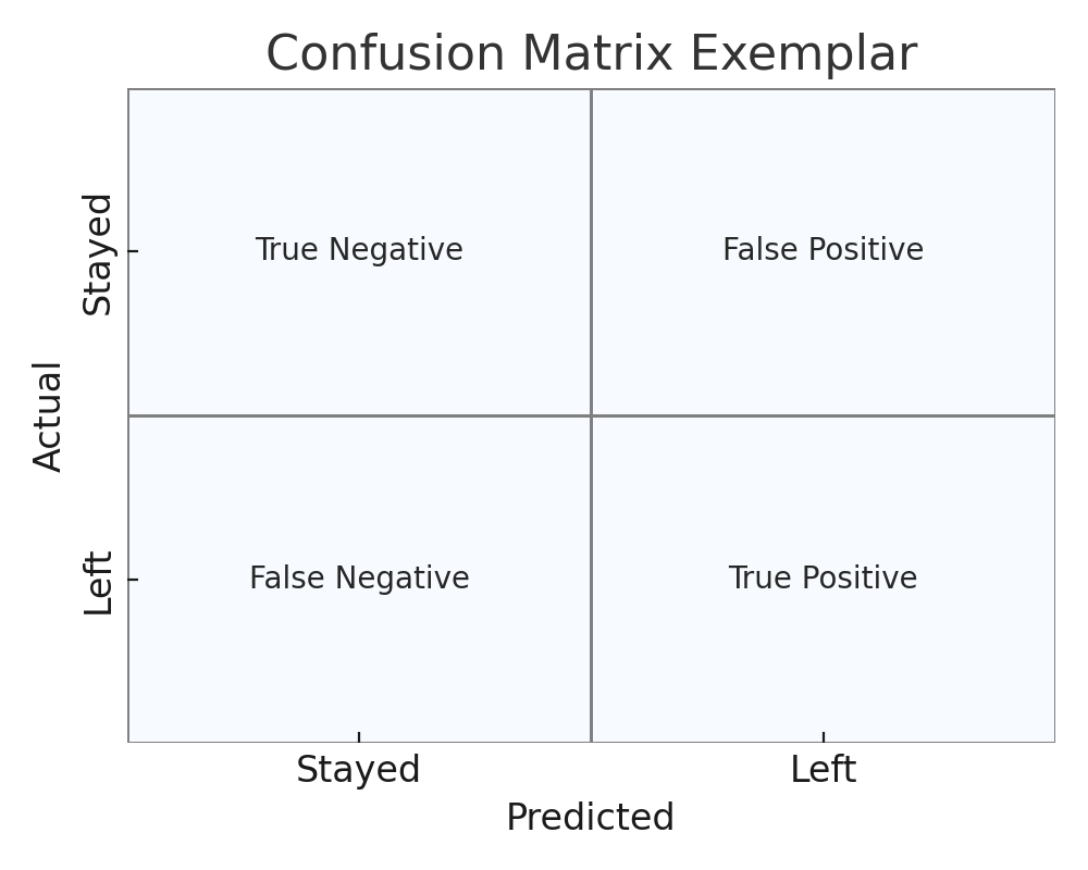
🔲 Model Confusion Matrices
Confusion matrices show how often the models got it right, and how they got it wrong. Here's what we cared about:
True Positives: Correctly flagged people who left
False Negatives: People who left, but the model missed (the worst outcome)
False Positives: People who stayed, but the model said they’d leave (not ideal, but tolerable)
Why prioritize catching leavers? Because hiring and onboarding are expensive. Better to offer a stay-bonus to someone who’d stay anyway than to lose someone you didn’t see coming.
I was okay crying wolf. I just didn’t want to miss the real wolves.

📝 Model Metrics
Below is each model’s precision, recall, and PR-AUC (Precision-Recall Area Under Curve), amongst other metrics. In short:
Recall tells us how many leavers we correctly flagged.
Precision tells us how many of our “they’ll leave” predictions were actually right.
PR-AUC tells us how well the model balances those two as we shift thresholds.
In the end, XGBoost won, the most cost-effective, best-performing, and the least prone to panic.
But the other models helped build understanding, especially Logistic Regression and Decision Tree, which offered valuable interpretability... to an extent.
| Model | Recall | F2 Score | F1 Score | Precision | Accuracy | PR AUC | ROC AUC | Features | Confusion Matrix |
|---|---|---|---|---|---|---|---|---|---|
| Logistic Regression | 0.934 | 0.847 | 0.743 | 0.618 | 0.891 | 0.744 | 0.948 | 14 | [[1639 218] [ 25 352]] |
| Decision Tree | 0.945 | 0.897 | 0.835 | 0.748 | 0.938 | 0.766 | 0.956 | 7 | [[1874 127] [ 22 376]] |
| Random Forest | 0.945 | 0.899 | 0.838 | 0.754 | 0.940 | 0.946 | 0.978 | 7 | [[1878 123] [ 22 376]] |
| XGBoost | 0.940 | 0.925 | 0.904 | 0.872 | 0.967 | 0.967 | 0.982 | 7 | [[1946 55] [ 24 374]] |
- Recall: Proportion of actual positives correctly identified (True Positives / [True Positives + False Negatives]).
- F₂-score: Harmonic mean prioritizing recall (80%) over precision (20%), tailored for this project's goals.
- F₁-score: Harmonic mean balancing precision and recall equally (50/50).
- Precision: Proportion of positive predictions that are correct (True Positives / [True Positives + False Positives]).
- Accuracy: Proportion of all predictions that are correct.
- PR AUC: Area under the precision-recall curve, the trade-off between precision and recall.
- ROC AUC: Probability the model is more confident (assigns a higher predicted probability) that a random leaver will leave than a random stayer will stay.
🕸️ The Interpretability Mirage: Logistic Regression and Multicollinearity
Logistic Regression has a fatal flaw: it assumes nice, clean, independent input features.
But real data isn’t that polite.
Enter multicollinearity, when two or more features are closely related. Think chocolate chips and chocolate chunks in a cookie recipe. Or sunlight and daylight hours when predicting plant growth. The model gets confused about who’s really responsible.
I checked this with Variance Inflation Factors (VIFs). Of course they were high (5 is troublesome). In every model I tried. Some variables were clearly stepping on each other’s toes. In the full feature model, some of that multicollinearity canceled itself out (weird, I know). But any time I removed a few features, like department, the problem got louder, not quieter.
So when my final selection criteria landed on a logistic model that double counted a few variables, I just shrugged. Interpretability was already out the window. Might as well go for predictive power.
| feature | VIF |
|---|---|
| satisfaction_level | 1.09 |
| last_evaluation | 1.15 |
| number_project | 1.25 |
| avg_monthly_hours | 1.18 |
| tenure | 1.13 |
| work_accident | 1.00 |
| promotion | 1.02 |
| salary | 1.02 |
| dept_IT | 4.71 |
| dept_RandD | 3.77 |
| dept_accounting | 3.38 |
| dept_hr | 3.37 |
| dept_management | 2.60 |
| dept_marketing | 3.51 |
| dept_product_mng | 3.58 |
| dept_sales | 12.99 |
| dept_support | 8.13 |
| dept_technical | 9.73 |
| feature | VIF |
|---|---|
| satisfaction_level | 6.92 |
| last_evaluation | 19.60 |
| number_project | 14.04 |
| avg_monthly_hours | 18.51 |
| tenure | 11.79 |
| promotion | 1.02 |
📉 Trade-Off Between Precision and Recall
Every model made trade-offs between false positives and false negatives. That trade-off is tunable using the classification threshold.
Recall = TP / (TP + FN): How well we catch actual leavers
Precision = TP / (TP + FP): How many predicted leavers really do leave
Below, you’ll see how Logistic Regression desperately boosts recall at the expense of precision, crying wolf far more often to catch every actual wolf. XGBoost, meanwhile, finds a much better balance.

📋 Model Mistakes: Who Got It Wrong, And How?
| Model | Total Misclassified | False Positives (FP) | False Negatives (FN) |
|---|---|---|---|
| Logistic Regression | 243 | 218 | 25 |
| Decision Tree | 149 | 127 | 22 |
| Random Forest | 145 | 123 | 22 |
| XGBoost | 79 | 55 | 24 |
Notes:
False Positives (FP): Predicted "Left", actually "Stayed"
False Negatives (FN): Predicted "Stayed", actually "Left"
Total Misclassified = FP + FN
I dug into where the mistakes happened. One illustrative case (below): employees with 3–4 years tenure and satisfaction under 0.5. Classic “gray area” employees. Decision Trees and Random Forests struggled here. XGBoost didn’t. It picked up on subtle interactions that others missed.

📊 Model Confidence in Its Mistakes
Models don’t actually say “Leave” or “Stay”. They say things like “72% chance of leaving.” The cutoff is usually 50%. But we can shift it.
So I looked at how confident the models were when they got it wrong.
Decision Tree? Loud and wrong. It made many high-confidence errors, saying someone was 90% likely to leave when they didn’t. Random Forest was similar but a touch less confident.
XGBoost? Still wrong sometimes, but with humility. Its misclassifications had a nice, balanced distribution. It knew what it didn’t know. Sometimes.

🧠 Final Verdict
So yes, XGBoost technically made about the same number of false negatives as Decision Tree and Random Forest. But it made way fewer false positives, and was far more measured in its predictions.
In the end, XGBoost is the best-performing model: confident when appropriate, humble when uncertain, and better than the rest at spotting those elusive leavers without constantly crying wolf.
The kind of model I’d trust with a retention budget.
Model Interpretation
Machine learning is an interpretable…?? Thing Label-er.
Now comes the part where we try to understand why the models made the decisions they did.
Interpretability is where things get... slippery. Logistic Regression is supposed to be our beacon of clarity, but multicollinearity clouded the glass. Decision Trees are still readable. Random Forest and XGBoost? Not so much, unless you squint, poke, prod, and apply a little Game Theory.
Let’s walk through what we can interpret.
🔍 Feature Importances
Let’s start with the basics: which features mattered most?
On the left, we have the Logistic Regression coefficients. Direction and magnitude show how each feature pushes the model toward “Stay” or “Leave.” Ignore the confusing bins (thanks again, multicollinearity) and the key insights still hold:
More tenure and more hours? Higher chance of leaving.
More satisfaction? More likely to stay.
On the right, XGBoost’s feature importances: a score from 0 to 1 based on how often and how effectively a feature was used across all those sequential decision trees.
Tenure led the pack, followed by satisfaction, number of projects, and hours.
The Burnout flag was surprisingly irrelevant, likely redundant with the other features.
Random Forest showed a similar importance pattern, suggesting a consensus among the more complex models.

🔥SHAP summary plot
SHAP values (SHapley Additive exPlanations) offer a more nuanced look into how features influenced individual predictions. Each row has a dot for every employee.
Color = feature value (red=high, blue=low)
X-axis = effect on prediction (negative = more likely to stay, positive = more likely to leave)
Highlights:
High satisfaction (very red) leans strongly toward “Stay.”
Extremely low satisfaction (light blue) tips strongly toward “Leave.
High tenure (red) leads to leave predictions, but the longest-tenured swing back to stay, echoing the EDA finding of long-term survivors.
Few projects (blue) = disengaged leavers. Too many (red) = burnout leavers.
Very high hours (red)? Classic burnout territory. And the opposite holds, with fewer hours liable to "Stay," and a jumble in the middle.
Some top evaluations (red) still leave. Meanwhile, lower-rated employees (blue) often stick around.
No surprise here: burnt-out, overwhelmed, and unhappy people quit—even if they’re doing a great job.
SHAP gives us a peek under the hood of the black box, just enough to see that it’s not totally opaque. As for how it works: something to do with cooperative game theory. “Because math,” basically. Calculus pixies.

🌳 Decision Tree: The Explainable One
Here’s where we can breathe a little easier. The Decision Tree lays everything out like a choose-your-own-adventure book.
Each split says:
What feature and threshold it used
Gini impurity (how mixed the groups are)
Samples at that node
Value: count of [Stay, Leave]
Class: the majority class at that node
You can read it top to bottom, each branch a path through the forest of logic.
All of these decisions—these splits—feed into the feature importances used by the more complex models like XGBoost.
Below the tree, you’ll find:
A summary of all splits
A scrollable outline from root to leaf, showing class counts and rules along the way

🌟 Primary Split:
- satisfaction_level ≤ 0.47 → More likely to Leave, especially with low tenure or high hours.
- satisfaction_level > 0.47 → More likely to Stay, especially if tenure is low and projects/hours are moderate.
🟥 If satisfaction_level ≤ 0.47:
📌 Tenure ≤ 4.5
- Tenure ≤ 2.5
- Very low satisfaction (≤ 0.15) and moderate-to-high hours → Left
- Else → Stayed
- Tenure > 2.5
- Low hours or low evaluation → Stayed
- High evaluation → Left
📌 Tenure > 4.5
- Very low satisfaction (≤ 0.11) → Left
- Else:
- Many projects or very high hours → Left
- Fewer projects and moderate hours → Stayed
✅ If satisfaction_level > 0.47:
📌 Tenure ≤ 4.5
- Hours ≤ 290.5
- Projects ≤ 6 → Stayed
- Projects > 6 → Left
- Hours > 290.5 → Left, regardless of satisfaction level (even if > 0.63)
📌 Tenure > 4.5
- Last eval ≤ 0.81
- Projects ≤ 6 → Stayed
- Projects > 6 → Left
- Last eval > 0.81
- Low hours → Stayed
- High hours → Left, unless tenure is very high (> 6.5)
🔑 Key Features Driving Decisions:
satisfaction_leveltenureaverage_monthly_hoursnumber_projectlast_evaluation
🌳 Scrollable Outline with Splits:
🧠 So... Can We Trust It?
XGBoost may not speak in clear rules, but it doesn't mean we can't understand its logic.
Logistic Regression tried to reason it out, but got caught in a web of overlapping variables.
Decision Tree laid out its logic like a flowchart, simple and straightforward.
SHAP values peeked under XGBoost’s hood, showing how features actually influenced decisions.
Feature importances ranked the key players, giving us a sense of what matters most.
Together, these tools help us decode a black box, turning it into something usable, even actionable.
XGBoost flags who is at risk.
EDA and the simpler models help explain why.
It’s not magic, and it’s not guesswork. It’s data-backed intelligence with practical implications.
In short: the model is complex. But the message to HR?
Keep your eye on the people most likely to leave—and do something about it.
Because replacing good people costs more than keeping them.
Conclusion
“All models are wrong, but some are useful.”
And that’s a thorough overview of the machine learning process. We started with a deceptively simple question:
Can we predict which employees are most likely to leave?
We began with Exploratory Data Analysis that revealed key patterns—particularly the relationship between satisfaction and tenure, which hinted at disengagement, burnout, and employee fatigue.
That insight led the way: guiding feature engineering, model selection, and business-aligned goals like maximizing recall while maintaining reasonable precision.
We tested multiple models, each with its strengths and flaws.

| Model | Recall | F2 Score | F1 Score | Precision | Accuracy | PR AUC | ROC AUC |
|---|---|---|---|---|---|---|---|
| XGBoost | 0.940 | 0.925 | 0.904 | 0.872 | 0.967 | 0.967 | 0.982 |
But XGBoost stood out. It was:
The most accurate overall.
The most balanced in confidence and error.
The most capable of flagging risk in the ambiguous middle ground: those 3–4 year employees whose dissatisfaction simmers quietly.
While it doesn’t deliver a simple checklist, it points us to the people who need attention and, when paired with insights from EDA and interpretable models, helps us figure out what action to take.
🏅 XGBoost Wins. Retention Wins.
The final takeaway?
The model works. It’s not perfect. But it’s smart. And it’s enough to help HR stay ahead of the curve, before the next resignation letter hits the desk.
Let’s keep our people. Salifort Motors runs better when it runs together. (I'll take that LinkedIn Influencer award now.)
Continue Exploring:
Appendix: Data Dictionaries
Original Dataset
After removing duplicates, the dataset contained 11,991 rows and 10 columns for the variables listed below.
Note: For more information about the data, refer to its source on Kaggle. The data has been repurposed and adapted for this project as part of the Google Advanced Data Analytics Capstone.
Variable |Description | -----|-----| satisfaction_level|Employee-reported job satisfaction level [0–1]| last_evaluation|Score of employee's last performance review [0–1]| number_project|Number of projects employee contributes to| average_monthly_hours|Average number of hours employee worked per month| time_spend_company|How long the employee has been with the company (years) Work_accident|Whether or not the employee experienced an accident while at work left|Whether or not the employee left the company promotion_last_5years|Whether or not the employee was promoted in the last 5 years Department|The employee's department salary|The employee's salary (U.S. dollars)
Logistic Regression with Binning and Feature Selection
This model uses a subset of the original features, applies binning to key variables, and drops department, salary, and work_accident.
| Variable | Description |
|---|---|
| satisfaction_level | Employee-reported job satisfaction level [0–1] |
| last_evaluation | Score of employee's last performance review [0–1] |
| number_project | Number of projects employee contributes to |
| average_monthly_hours | Average number of hours employee worked per month |
| tenure | How long the employee has been with the company (years) |
| promotion_last_5years | Whether or not the employee was promoted in the last 5 years |
| satisfaction_bin_medium | Binary indicator: satisfaction_level is medium (> 0.4 and ≤ 0.7) |
| satisfaction_bin_high | Binary indicator: satisfaction_level is high (> 0.7) |
| hours_bin_medium | Binary indicator: average_monthly_hours is medium (> 160 and ≤ 240) |
| hours_bin_high | Binary indicator: average_monthly_hours is high (> 240) |
| projects_bin_medium | Binary indicator: number_project is medium (> 2 and ≤ 5) |
| projects_bin_high | Binary indicator: number_project is high (> 5) |
| tenure_bin_mid | Binary indicator: tenure is mid (> 3 and ≤ 5 years) |
| tenure_bin_long | Binary indicator: tenure is long (> 5 years) |
- All binned features are one-hot encoded, with the first category dropped (i.e., "low" or "short" is the reference).
Tree-Based Models — "Core + Burnout" Features
This model uses a focused set of original features plus an engineered "burnout" flag.
| Variable | Description |
|---|---|
| satisfaction_level | Employee-reported job satisfaction level [0–1] |
| last_evaluation | Score of employee's last performance review [0–1] |
| number_project | Number of projects employee contributes to |
| average_monthly_hours | Average number of hours employee worked per month |
| tenure | How long the employee has been with the company (years) |
| promotion_last_5years | Whether or not the employee was promoted in the last 5 years |
| burnout | Flag: True if (number_project ≥ 6 or average_monthly_hours ≥ 240) and satisfaction_level ≤ 0.3 |
- The "burnout" feature is a logical flag engineered to capture high-risk, overworked, and dissatisfied employees.