
# Import packages
import time
import joblib
import os
import warnings

warnings.filterwarnings("ignore")

import pandas as pd
import numpy as np
import math

import matplotlib.pyplot as plt
import seaborn as sns
from sklearn.tree import plot_tree

from IPython.display import Image, display, HTML

from sklearn.model_selection import (
    StratifiedKFold,
    cross_val_predict,
    GridSearchCV,
    RandomizedSearchCV,
    train_test_split,
)
from sklearn.pipeline import Pipeline
from sklearn.preprocessing import StandardScaler
from sklearn.preprocessing import FunctionTransformer

from sklearn.linear_model import LogisticRegression
from sklearn.tree import DecisionTreeClassifier
from sklearn.ensemble import RandomForestClassifier
from xgboost import XGBClassifier

from statsmodels.stats.outliers_influence import variance_inflation_factor

from sklearn.metrics import (
    accuracy_score,
    precision_score,
    recall_score,
    f1_score,
    roc_auc_score,
    confusion_matrix,
    fbeta_score,
    average_precision_score,
)


# get initial time, for measuring performance at the end
nb_start_time = time.time()


# Load dataset into a dataframe
df0 = pd.read_csv("../resources/HR_capstone_dataset.csv")


# Display first few rows of the dataframe
df0.head()


# Gather basic information about the data
df0.info()

<class 'pandas.core.frame.DataFrame'>
RangeIndex: 14999 entries, 0 to 14998
Data columns (total 10 columns):
 #   Column                 Non-Null Count  Dtype  
---  ------                 --------------  -----  
 0   satisfaction_level     14999 non-null  float64
 1   last_evaluation        14999 non-null  float64
 2   number_project         14999 non-null  int64  
 3   average_montly_hours   14999 non-null  int64  
 4   time_spend_company     14999 non-null  int64  
 5   Work_accident          14999 non-null  int64  
 6   left                   14999 non-null  int64  
 7   promotion_last_5years  14999 non-null  int64  
 8   Department             14999 non-null  object 
 9   salary                 14999 non-null  object 
dtypes: float64(2), int64(6), object(2)
memory usage: 1.1+ MB


# Department value counts and percent
dept_counts = df0.Department.value_counts()
dept_percent = df0.Department.value_counts(normalize=True) * 100
dept_summary = pd.DataFrame({"Count": dept_counts, "Percent": dept_percent.round(2)})
print("Department value counts and percent:\n", dept_summary)

# Salary value counts and percent
salary_counts = df0.salary.value_counts()
salary_percent = df0.salary.value_counts(normalize=True) * 100
salary_summary = pd.DataFrame(
    {"Count": salary_counts, "Percent": salary_percent.round(2)}
)
print("\nSalary value counts and percent:\n", salary_summary)

Department value counts and percent:
              Count  Percent
Department                 
sales         4140    27.60
technical     2720    18.13
support       2229    14.86
IT            1227     8.18
product_mng    902     6.01
marketing      858     5.72
RandD          787     5.25
accounting     767     5.11
hr             739     4.93
management     630     4.20

Salary value counts and percent:
         Count  Percent
salary                
low      7316    48.78
medium   6446    42.98
high     1237     8.25


# Gather descriptive statistics about the data
df0.describe()


df0.columns

Index(['satisfaction_level', 'last_evaluation', 'number_project',
       'average_montly_hours', 'time_spend_company', 'Work_accident', 'left',
       'promotion_last_5years', 'Department', 'salary'],
      dtype='object')


# Rename columns as needed
df0.rename(
    columns={
        "Department": "department",
        "Work_accident": "work_accident",
        "average_montly_hours": "average_monthly_hours",
        "time_spend_company": "tenure",
    },
    inplace=True,
)


# Display all column names after the update
df0.columns

Index(['satisfaction_level', 'last_evaluation', 'number_project',
       'average_monthly_hours', 'tenure', 'work_accident', 'left',
       'promotion_last_5years', 'department', 'salary'],
      dtype='object')


# Check for missing values
df0.isna().sum()

satisfaction_level       0
last_evaluation          0
number_project           0
average_monthly_hours    0
tenure                   0
work_accident            0
left                     0
promotion_last_5years    0
department               0
salary                   0
dtype: int64


# Check for duplicates
df0.duplicated().sum()

3008


# Inspect some rows containing duplicates as needed
df0[df0.duplicated()].head()


# Drop duplicates and save resulting dataframe in a new variable as needed
df = df0.drop_duplicates()


# Display first few rows of new dataframe as needed
print(df.info())
df.head()

<class 'pandas.core.frame.DataFrame'>
Index: 11991 entries, 0 to 11999
Data columns (total 10 columns):
 #   Column                 Non-Null Count  Dtype  
---  ------                 --------------  -----  
 0   satisfaction_level     11991 non-null  float64
 1   last_evaluation        11991 non-null  float64
 2   number_project         11991 non-null  int64  
 3   average_monthly_hours  11991 non-null  int64  
 4   tenure                 11991 non-null  int64  
 5   work_accident          11991 non-null  int64  
 6   left                   11991 non-null  int64  
 7   promotion_last_5years  11991 non-null  int64  
 8   department             11991 non-null  object 
 9   salary                 11991 non-null  object 
dtypes: float64(2), int64(6), object(2)
memory usage: 1.0+ MB
None


# Boxplot of `average_monthly_hours` to visualize distribution and detect outliers
plt.figure(figsize=(6, 2))
sns.boxplot(x=df["average_monthly_hours"])
plt.title("Boxplot of Average Monthly Hours")
plt.xlabel("Average Monthly Hours")
plt.show()


# Create a boxplot to visualize distribution of `tenure` and detect any outliers
plt.figure(figsize=(6, 2))
sns.boxplot(x=df["tenure"])
plt.title("Boxplot of Tenure")
plt.xlabel("Tenure")
plt.show()


# Determine the number of rows containing outliers
q1 = df.tenure.quantile(0.25)
q3 = df.tenure.quantile(0.75)
iqr = q3 - q1
upper_bound = q3 + 1.5 * iqr

print(f"Upper bound for outliers in tenure: {upper_bound}")

# Filter the dataframe to find outliers
outliers = df[df.tenure > upper_bound]

# Display the number of outliers
print(f"Number of tenure outliers: {len(outliers)}")
print(f"Outliers percentage of total: {len(outliers) / len(df) * 100:.2f}%")
df.tenure.value_counts()

Upper bound for outliers in tenure: 5.5
Number of tenure outliers: 824
Outliers percentage of total: 6.87%

tenure
3     5190
2     2910
4     2005
5     1062
6      542
10     107
7       94
8       81
Name: count, dtype: int64


# Get numbers of people who left vs. stayed
# Get percentages of people who left vs. stayed
left_counts = df.left.value_counts()
left_percent = df.left.value_counts(normalize=True) * 100

left_summary = pd.DataFrame({"Count": left_counts, "Percent": left_percent.round(2)})

left_summary.index = left_summary.index.map({0: "Stayed", 1: "Left"})
left_summary


# Pairplot to visualize relationships between features
sns.pairplot(df, hue="left", diag_kind="kde", plot_kws={"alpha": 0.1})
plt.show()


# Boxplots to visualize distributions of numerical features by `left`
numerical_cols = [
    "satisfaction_level",
    "last_evaluation",
    "number_project",
    "average_monthly_hours",
    "tenure",
]

plt.figure(figsize=(15, 8))
for i, col in enumerate(numerical_cols, 1):
    plt.subplot(2, 3, i)
    sns.boxplot(x="left", y=col, data=df)
    plt.title(f"{col} by left")
plt.tight_layout()
plt.show()


# Violin plots to visualize distributions of numerical features by `left`
numerical_cols = [
    "satisfaction_level",
    "last_evaluation",
    "number_project",
    "average_monthly_hours",
    "tenure",
]

plt.figure(figsize=(15, 8))
for i, col in enumerate(numerical_cols, 1):
    plt.subplot(2, 3, i)
    sns.violinplot(x="left", y=col, data=df, inner="box")
    plt.title(f"{col} by left")
plt.tight_layout()
plt.show()


# Histograms to visualize distributions of numerical features
numerical_cols = [
    "satisfaction_level",
    "last_evaluation",
    "number_project",
    "average_monthly_hours",
    "tenure",
]

plt.figure(figsize=(15, 8))
for i, col in enumerate(numerical_cols, 1):
    plt.subplot(2, 3, i)
    sns.histplot(
        data=df,
        x=col,
        hue="left",
        kde=True,
        element="step",
        stat="density",
        common_norm=False,
    )
    plt.title(f"{col} by left")
plt.tight_layout()
plt.show()


# Histograms to visualize distributions of numerical features (showing true count)
numerical_cols = [
    "satisfaction_level",
    "last_evaluation",
    "number_project",
    "average_monthly_hours",
    "tenure",
]

plt.figure(figsize=(15, 8))
for i, col in enumerate(numerical_cols, 1):
    plt.subplot(2, 3, i)
    sns.histplot(data=df, x=col, hue="left", kde=True, element="step", stat="count")
    plt.title(f"{col} by left")
plt.tight_layout()
plt.show()


# Plot satisfaction vs. hours worked, colored by left
plt.figure(figsize=(8, 6))
sns.scatterplot(
    data=df,
    x="satisfaction_level",
    y="average_monthly_hours",
    hue="left",
    alpha=0.3,
)
plt.title("Satisfaction vs. Average Monthly Hours")
plt.xlabel("Satisfaction Level")
plt.ylabel("Average Monthly Hours")
plt.legend(loc="upper right", labels=["Left", "Stayed"])
plt.show()


# Plot satisfaction level vs last evaluation, colored by left
plt.figure(figsize=(8, 6))
sns.scatterplot(
    data=df,
    x="satisfaction_level",
    y="last_evaluation",
    hue="left",
    alpha=0.3,
)
plt.title("Satisfaction Level vs. Last Evaluation")
plt.xlabel("Satisfaction Level")
plt.ylabel("Last Evaluation")
plt.legend(loc="lower right", labels=["Left", "Stayed"])
plt.show()


# Get mean and median satisfaction level for those who left vs. stayed
mean_satisfaction = df.groupby("left")["satisfaction_level"].mean()
median_satisfaction = df.groupby("left")["satisfaction_level"].median()

satisfaction_summary = pd.DataFrame(
    {"Mean": mean_satisfaction, "Median": median_satisfaction}
)

satisfaction_summary.index = satisfaction_summary.index.map({0: "Stayed", 1: "Left"})
satisfaction_summary


# Plot last evaluation vs. average monthly hours, colored by left
plt.figure(figsize=(8, 6))
sns.scatterplot(
    data=df,
    x="last_evaluation",
    y="average_monthly_hours",
    hue="left",
    alpha=0.3,
)
plt.title("Last Evaluation vs. Average Monthly Hours")
plt.xlabel("Last Evaluation")
plt.ylabel("Average Monthly Hours")
plt.legend(loc="upper right", labels=["Left", "Stayed"])
plt.show()


# Bar plot of tenure by left
plt.figure(figsize=(8, 6))
sns.countplot(data=df, x="tenure", hue="left")
plt.title("Count of Employees by Tenure and Left")
plt.xlabel("Tenure")
plt.ylabel("Count")
plt.legend(title="Left", loc="upper right", labels=["Stayed", "Left"])
plt.show()


# Get total and percentage of employees by tenure and left
tenure_counts = df.groupby(["tenure", "left"]).size().unstack(fill_value=0)
tenure_percent = tenure_counts.div(tenure_counts.sum(axis=1), axis=0) * 100
tenure_summary = pd.DataFrame(
    {"Count": tenure_counts.stack(), "Percent": tenure_percent.stack()}
).reset_index()
tenure_summary.columns = ["Tenure", "Left", "Count", "Percent"]
tenure_summary["Left"] = tenure_summary["Left"].map({0: "Stayed", 1: "Left"})
tenure_summary


# Boxplot of tenure vs average monthly hours, split by left
plt.figure(figsize=(8, 6))
sns.boxplot(data=df, x="tenure", y="average_monthly_hours", hue="left")
plt.title("Average Monthly Hours by Tenure and Left")
plt.xlabel("Tenure")
plt.ylabel("Average Monthly Hours")
plt.legend(title="Left", loc="upper right", labels=["Stayed", "Left"])
plt.show()


# Box plot of tenure vs satisfaction level, split by left
plt.figure(figsize=(8, 6))
sns.boxplot(data=df, x="tenure", y="satisfaction_level", hue="left")
plt.title("Satisfaction Level by Tenure and Left")
plt.xlabel("Tenure")
plt.ylabel("Satisfaction Level")
plt.legend(title="Left", loc="upper right", labels=["Stayed", "Left"])
plt.show()


# Bar plot of department vs. left
plt.figure(figsize=(8, 6))
sns.countplot(
    data=df,
    x="department",
    hue="left",
)
plt.title("Count of Employees by Department and Left")
plt.xlabel("Department")
plt.ylabel("Count")
plt.legend(loc="upper right", labels=["Stayed", "Left"])
plt.xticks(rotation=45)
plt.show()


# Get total and percentage of employees by department and left
dept_counts = df.groupby(["department", "left"]).size().unstack(fill_value=0)

# Calculate percentages within each department (row-wise)
dept_percent = dept_counts.div(dept_counts.sum(axis=1), axis=0) * 100

# Reshape for easier viewing: melt to long format
dept_summary = (
    dept_counts.join(dept_percent, lsuffix="_count", rsuffix="_percent")
    .reset_index()
    .melt(id_vars="department", value_name="Value", var_name="Status")
)

# Split Status into Left and Item
dept_summary[["Left", "Item"]] = dept_summary["Status"].str.extract(
    r"(\d)_(count|percent)"
)
dept_summary["Left"] = dept_summary["Left"].map({"0": "Stayed", "1": "Left"})

# Pivot so each row is department + Left, with Count and Percent columns
dept_summary = (
    dept_summary.pivot_table(
        index=["department", "Left"], columns="Item", values="Value"
    )
    .reset_index()
    .rename(columns={"count": "Count", "percent": "Percent"})
)

# Round Percent
dept_summary["Percent"] = dept_summary["Percent"].round(2)

dept_summary


# Bar plot of salary vs. left
plt.figure(figsize=(8, 6))
sns.countplot(
    data=df,
    x="salary",
    hue="left",
)
plt.title("Count of Employees by Salary and Left")
plt.xlabel("Salary")
plt.ylabel("Count")
plt.legend(loc="upper right", labels=["Stayed", "Left"])
plt.xticks(rotation=45)
plt.show()


# Get total and percentage of employees by salary and left
salary_counts = df.groupby(["salary", "left"]).size().unstack(fill_value=0)
salary_percent = salary_counts.div(salary_counts.sum(axis=1), axis=0) * 100

salary_summary = (
    salary_counts.join(salary_percent, lsuffix="_count", rsuffix="_percent")
    .reset_index()
    .melt(id_vars="salary", value_name="Value", var_name="Status")
)

# Split Status into Left and Item
salary_summary[["Left", "Item"]] = salary_summary["Status"].str.extract(
    r"(\d)_(count|percent)"
)
salary_summary["Left"] = salary_summary["Left"].map({"0": "Stayed", "1": "Left"})

# Pivot so each row is salary + Left, with Count and Percent columns
salary_summary = (
    salary_summary.pivot_table(index=["salary", "Left"], columns="Item", values="Value")
    .reset_index()
    .rename(columns={"count": "Count", "percent": "Percent"})
)
salary_summary["Percent"] = salary_summary["Percent"].round(2)
salary_summary


# Bar plot of promotion last 5 years vs. left
plt.figure(figsize=(8, 6))
sns.countplot(
    data=df,
    x="promotion_last_5years",
    hue="left",
)
plt.title("Count of Employees by Promotion Last 5 Years and Left")
plt.xlabel("Promotion Last 5 Years")
plt.ylabel("Count")
plt.legend(loc="upper right", labels=["Stayed", "Left"])
plt.show()


# Scatter plot average monthly hours vs. promotion last 5 years, colored by left
plt.figure(figsize=(8, 3))
sns.scatterplot(
    data=df,
    x="average_monthly_hours",
    y="promotion_last_5years",
    hue="left",
    alpha=0.3,
)
plt.title("Average Monthly Hours vs. Promotion Last 5 Years")
plt.xlabel("Average Monthly Hours")
plt.ylabel("Promotion Last 5 Years")
plt.legend(loc="center right", labels=["Left", "Stayed"])
plt.show()


# Bar plot of promotion last 5 years and tenure
plt.figure(figsize=(8, 6))
sns.countplot(
    data=df,
    x="tenure",
    hue="promotion_last_5years",
)
plt.title("Count of Employees by Promotion Last 5 Years and Tenure")
plt.xlabel("Promotion Last 5 Years")
plt.ylabel("Count")
plt.legend(loc="upper right", labels=["Stayed", "Left"])
plt.show()


# Bar plot of work accident vs. left
plt.figure(figsize=(8, 6))
sns.countplot(
    data=df,
    x="work_accident",
    hue="left",
)
plt.title("Count of Employees by Work Accident and Left")
plt.xlabel("Work Accident")
plt.ylabel("Count")
plt.legend(loc="upper right", labels=["Stayed", "Left"])
plt.show()


# Count and percentage for work_accident and left (work_accident first)
cross_counts = df.groupby(["work_accident", "left"]).size().unstack(fill_value=0)
cross_percent = cross_counts.div(cross_counts.sum(axis=1), axis=0) * 100

summary = (
    cross_counts.astype(int)
    .join(cross_percent.round(2), lsuffix="_count", rsuffix="_percent")
    .reset_index()
    .melt(id_vars="work_accident", value_name="Value", var_name="Status")
)

# Split Status into Left and Item
summary[["left", "Item"]] = summary["Status"].str.extract(r"(\d)_(count|percent)")
summary["left"] = summary["left"].map({"0": "Stayed", "1": "Left"})
summary["work_accident"] = summary["work_accident"].map({0: "No", 1: "Yes"})

# Pivot for easier viewing
summary = (
    summary.pivot_table(index=["work_accident", "left"], columns="Item", values="Value")
    .reset_index()
    .rename(columns={"count": "Count", "percent": "Percent"})
)

summary


# Bar plot of number of projects vs. left
plt.figure(figsize=(8, 6))
sns.countplot(
    data=df,
    x="number_project",
    hue="left",
)
plt.title("Count of Employees by Number of Projects and Left")
plt.xlabel("Number of Projects")
plt.ylabel("Count")
plt.legend(loc="upper right", labels=["Stayed", "Left"])
plt.show()


# Count and percentage for number_project and left (number_project first)
cross_counts = df.groupby(["number_project", "left"]).size().unstack(fill_value=0)
cross_percent = cross_counts.div(cross_counts.sum(axis=1), axis=0) * 100

summary = (
    cross_counts.astype(int)
    .join(cross_percent.round(2), lsuffix="_count", rsuffix="_percent")
    .reset_index()
    .melt(id_vars="number_project", value_name="Value", var_name="Status")
)

# Split Status into Left and Item
summary[["left", "Item"]] = summary["Status"].str.extract(r"(\d)_(count|percent)")
summary["left"] = summary["left"].map({"0": "Stayed", "1": "Left"})

# Pivot for easier viewing
summary = (
    summary.pivot_table(
        index=["number_project", "left"], columns="Item", values="Value"
    )
    .reset_index()
    .rename(columns={"count": "Count", "percent": "Percent"})
)

summary


# Boxplot of number of projects vs. average monthly hours, split by left
plt.figure(figsize=(8, 6))
sns.boxplot(
    data=df,
    x="number_project",
    y="average_monthly_hours",
    hue="left",
)
plt.title("Number of Projects vs. Average Monthly Hours")
plt.xlabel("Number of Projects")
plt.ylabel("Average Monthly Hours")
plt.legend(loc="lower right")
plt.show()


# Boxplot of satisfaction level vs number of projects, split by left
plt.figure(figsize=(8, 6))
sns.boxplot(
    data=df,
    x="number_project",
    y="satisfaction_level",
    hue="left",
)
plt.title("Satisfaction Level vs. Number of Projects")
plt.xlabel("Number of Projects")
plt.ylabel("Satisfaction Level")
plt.legend(loc="upper right")
plt.show()


# Bar plot of number of projects vs salary
plt.figure(figsize=(8, 6))
sns.countplot(
    data=df,
    x="number_project",
    hue="salary",
)
plt.title("Count of Employees by Number of Projects and Salary")
plt.xlabel("Number of Projects")
plt.ylabel("Count")
plt.legend(loc="upper right", labels=["Low", "Medium", "High"])
plt.show()


# Bar plot of number of projects vs salary, separated by left
sns.catplot(
    data=df,
    x="number_project",
    hue="salary",
    col="left",
    kind="count",
    height=6,
    aspect=1,
)
plt.subplots_adjust(top=0.8)
plt.suptitle("Count of Employees by Number of Projects, Salary, and Left Status")
plt.show()


# Correlation matrix
plt.figure(figsize=(10, 8))
sns.heatmap(
    df.select_dtypes(include=[np.number]).corr(),
    annot=True,
    fmt=".2f",
    cmap="coolwarm",
    square=True,
    cbar_kws={"shrink": 0.8},
)
plt.title("Correlation Matrix")
plt.show()


# set evaluation metric
scoring = "recall"


# for XGBoost eval_metric
def get_xgb_eval_metric(scoring):
    mapping = {
        "roc_auc": "auc",  # area under ROC curve
        "accuracy": "error",  # classification error rate
        "f1": "logloss",  # logarithmic loss (not F1, but closest available)
        "precision": "logloss",  # no direct precision metric, logloss is a common fallback
        "recall": "logloss",  # no direct recall metric, logloss is a common fallback
    }
    return mapping.get(scoring, "auc")  # default to 'auc' if not found


# copy the dataframe to avoid modifying the original
df_enc = df.copy()

# encode salary as ordinal
df_enc["salary"] = df_enc["salary"].map({"low": 0, "medium": 1, "high": 2})

# encode department as dummies
df_enc = pd.get_dummies(df_enc, columns=["department"])

# confirm the changes
print("Original salary values:\n", df["salary"].value_counts())
print("\nEncoded salary values:\n", df_enc["salary"].value_counts())
df_enc.columns

Original salary values:
 salary
low       5740
medium    5261
high       990
Name: count, dtype: int64

Encoded salary values:
 salary
0    5740
1    5261
2     990
Name: count, dtype: int64

Index(['satisfaction_level', 'last_evaluation', 'number_project',
       'average_monthly_hours', 'tenure', 'work_accident', 'left',
       'promotion_last_5years', 'salary', 'department_IT', 'department_RandD',
       'department_accounting', 'department_hr', 'department_management',
       'department_marketing', 'department_product_mng', 'department_sales',
       'department_support', 'department_technical'],
      dtype='object')


# split the data into features and target variable for tree-based models
X = df_enc.drop(columns=["left"])
y = df_enc["left"]

# split the data into training and testing sets
X_train, X_test, y_train, y_test = train_test_split(
    X, y, test_size=0.2, random_state=42, stratify=y
)

# scale_pos_weight for XGBoost (ratio of negative to positive class in training set)
scale_pos_weight_value = (y_train == 0).sum() / (y_train == 1).sum()


# split the data into features and target variable for logistic regression
# remove outliers from tenure for logistic regression
df_enc_lr = df_enc.copy()

"""
outliers defined waaaaaay up above, 
at end of inital data exploration and cleaning
code not needed here, but copied for reference
"""
# q1 = df.tenure.quantile(0.25)
# q3 = df.tenure.quantile(0.75)
# iqr = q3 - q1
# upper_bound = q3 + 1.5 * iqr

# remove outliers
df_enc_lr = df_enc_lr[df_enc_lr.tenure <= upper_bound]

X_lr = df_enc_lr.drop(columns=["left"])
y_lr = df_enc_lr["left"]

# split the data into training and testing sets for logistic regression
X_train_lr, X_test_lr, y_train_lr, y_test_lr = train_test_split(
    X_lr, y_lr, test_size=0.2, random_state=42, stratify=y_lr
)


def make_models_config(
    models,
    X_train,
    y_train,
    feature_func=None,  # can be a function, list, dict, or None
    param_grids=None,
    scaler=None,
    name_suffix="",
):
    """
    Build models_config for run_model_evaluation.
    - models: dict of {name: estimator}
    - X_train, y_train: training data
    - feature_func: function, list of functions, dict of {name: func}, or None
    - param_grids: dict of {name: param_grid} (or None for empty)
    - scaler: sklearn transformer (e.g., StandardScaler) or None
    - name_suffix: string to append to model name
    """
    configs = []
    for name, model in models.items():
        # order of steps matters, features first, then scaler, then model
        steps = []

        # determine which feature_func to use for this model
        func = None
        if isinstance(feature_func, dict):  # dict of {name: func}
            func = feature_func.get(name)
        elif callable(feature_func) or isinstance(feature_func, list):
            func = feature_func
        # handles a list of feature functions (apply in sequence), or a single function
        if func is not None:
            if isinstance(func, list):
                for i, f in enumerate(func):
                    steps.append((f"features_{i+1}", FunctionTransformer(f)))
            else:
                steps.append(("features", FunctionTransformer(func)))

        # add scaler if provided
        if scaler is not None:
            steps.append(("scaler", scaler))

        # add model
        steps.append(("model", model))

        # create the pipeline
        pipe = Pipeline(steps)

        # add parameter grid if provided
        param_grid = {}
        if isinstance(param_grids, dict):
            param_grid = param_grids.get(name, {})

        # add model configuration to the list
        configs.append(
            {
                "name": f"{name}{name_suffix}",
                "X_train": X_train,
                "y_train": y_train,
                "pipeline": pipe,
                "param_grid": param_grid,
            }
        )
    return configs


def run_model_evaluation(
    models_config,
    results_df=None,
    scoring="recall",
    save_model=False,
    search_type="grid",
    n_iter=20,
):
    """
    Run model training and evaluation for a list of model configurations using cross-validated hyperparameter search.

    For each model configuration, performs hyperparameter tuning (GridSearchCV or RandomizedSearchCV),
    fits the best pipeline, evaluates cross-validated performance metrics, and optionally saves the best model.

    Parameters:
        models_config (list of dict): List of model configurations, each containing:
            - 'name': Model name (str)
            - 'X_train': Training features (pd.DataFrame or np.ndarray)
            - 'y_train': Training labels (pd.Series or np.ndarray)
            - 'pipeline': sklearn Pipeline object
            - 'param_grid': dict of hyperparameters for search
        results_df (pd.DataFrame or None): Existing results DataFrame to append to, or None to create a new one.
        scoring (str): Scoring metric for model selection (e.g., 'recall', 'accuracy', 'roc_auc').
        save_model (bool): If True, saves the best model pipeline to disk for each configuration.
        search_type (str): 'grid' for GridSearchCV, 'random' for RandomizedSearchCV.
        n_iter (int): Number of parameter settings sampled for RandomizedSearchCV (ignored for grid search).

    Returns:
        pd.DataFrame: Results DataFrame with model name, metrics (recall, f1, roc_auc, precision, accuracy),
                      number of features, best hyperparameters, best CV score, confusion matrix, and search time.

    Notes:
        - Uses stratified 5-fold cross-validation for both hyperparameter search and out-of-fold predictions.
        - Calculates metrics on cross-validated predictions for robust performance estimates.
        - Handles models that do not support predict_proba for ROC AUC gracefully.
        - Saves models to '../results/saved_models/' if save_model=True.
    """
    if results_df is None:
        results_df = pd.DataFrame(
            columns=[
                "model",
                "recall",
                "f2",  # 80% recall, 20% precision (metric created to weigh recall more heavily)
                "f1",
                "pr_auc",
                "roc_auc",
                "precision",
                "accuracy",
                "features",
                "best_params",
                "cv_best_score",
                "conf_matrix",
                "search_time",
            ]
        )

    # ensure cross-validation is stratified for balanced class distribution
    cv = StratifiedKFold(n_splits=5, shuffle=True, random_state=42)

    for cfg in models_config:
        # time the model training and evaluation
        start_time = time.time()
        print(f"Running model: {cfg['name']}...")

        # conditional to choose search type, instantiate the appropriate search class
        if search_type == "random":
            grid = RandomizedSearchCV(
                cfg["pipeline"],
                cfg["param_grid"],
                n_iter=n_iter,
                cv=cv,
                scoring=scoring,
                n_jobs=-1,
                verbose=2,
                random_state=42,
            )
        else:
            grid = GridSearchCV(
                cfg["pipeline"],
                cfg["param_grid"],
                cv=cv,
                scoring=scoring,
                n_jobs=-1,
                verbose=2,
            )

        # fit the grid search to the training data
        grid.fit(cfg["X_train"], cfg["y_train"])

        # print the execution time
        end_time = time.time()
        search_time = end_time - start_time
        print(f"Execution time for {cfg['name']}: {search_time:.2f} seconds")

        # get the best model and its parameters
        best_model = grid.best_estimator_
        print(f"Best parameters for {cfg['name']}: {grid.best_params_}")
        print(f"Best score for {cfg['name']}: {grid.best_score_:.4f} ({scoring})")

        # --- get the number of features after all pipeline steps ---
        # try to transform X_train through all steps except the final estimator
        try:
            if hasattr(best_model, "named_steps"):
                # Remove the final estimator step
                steps = list(best_model.named_steps.items())
                if len(steps) > 1:
                    # Remove last step (the model)
                    feature_pipeline = Pipeline(steps[:-1])
                    X_transformed = feature_pipeline.transform(cfg["X_train"])
                    n_features = X_transformed.shape[1]
                else:
                    n_features = cfg["X_train"].shape[1]
            else:
                n_features = cfg["X_train"].shape[1]
        except Exception as e:
            print(f"Could not determine number of features: {e}")
            n_features = cfg["X_train"].shape[1]

        # conditional to save the best model
        if save_model:
            model_path = f"../results/saved_models/{cfg['name'].replace(' ', '_').lower()}.joblib"
            joblib.dump(best_model, model_path)
            print(f"Model {cfg['name']} saved successfully.\n")
        else:
            print(f"Model {cfg['name']} not saved. Set save_model=True to save it.\n")

        # make predictions using cross-validation to generate out-of-fold predictions for each training sample
        # translation:
        # substitute for setting aside a validation set
        # takes more time, but provides better estimates of model performance
        # it makes a prediction for each sample in the training set, using a different fold of the data for each prediction...
        # ...the fold where the sample is not included in the 80% training set (the sample is in the 20%)
        y_pred = cross_val_predict(
            best_model, cfg["X_train"], cfg["y_train"], cv=cv, n_jobs=-1
        )

        # # check misclassified cases for further analysis
        # print(f"Misclassified cases for {cfg['name']}:")
        # misclassified = cfg['X_train'].copy()
        # misclassified['actual'] = cfg["y_train"]
        # misclassified['predicted'] = y_pred
        # misclassified = misclassified[misclassified['actual'] != misclassified['predicted']]

        # # Show counts of each type of misclassification
        # counts = misclassified.groupby(['actual', 'predicted']).size().rename('count')
        # print("\nMisclassification counts:")
        # print(counts)
        # print()

        # # Show .describe() for each group, side by side
        # pd.set_option('display.max_columns', None)
        # for (actual, predicted), group in misclassified.groupby(['actual', 'predicted']):
        #     label_map = {0: "Stayed", 1: "Left"}
        #     print(f"--- Misclassified: Actual={label_map.get(actual, actual)}, Predicted={label_map.get(predicted, predicted)} (n={len(group)}) ---")
        #     print(group.describe().T)
        #     print()
        # pd.reset_option('display.max_columns')
        # print("\n")

        # calculate the ROC AUC score, need predicted probabilities (not just class labels, but confidence in those labels)
        # try / except block to handle models that do not support predict_proba (e.g., SVC)
        try:
            y_proba = cross_val_predict(
                best_model,
                cfg["X_train"],
                cfg["y_train"],
                cv=cv,
                method="predict_proba",
                n_jobs=-1,
            )
            roc_auc = roc_auc_score(cfg["y_train"], y_proba[:, 1])
            pr_auc = average_precision_score(cfg["y_train"], y_proba[:, 1])
        except (AttributeError, ValueError):
            roc_auc = np.nan
            pr_auc = np.nan
            print(f"Model {cfg['name']} does not support predict_proba.")

        # save results in the results dataframe
        results_df.loc[len(results_df)] = {
            "model": cfg["name"],
            "features": n_features,
            "accuracy": accuracy_score(cfg["y_train"], y_pred),
            "precision": precision_score(cfg["y_train"], y_pred),
            "recall": recall_score(cfg["y_train"], y_pred),
            "f1": f1_score(cfg["y_train"], y_pred),
            "f2": fbeta_score(
                cfg["y_train"], y_pred, beta=2
            ),  # 80% recall, 20% precision (ratio is "beta squared : 1", b^2:1, 2^2:1, 4:1)
            "roc_auc": roc_auc,
            "pr_auc": pr_auc,
            "conf_matrix": confusion_matrix(cfg["y_train"], y_pred).tolist(),
            "best_params": grid.best_params_,
            "cv_best_score": grid.best_score_,
            "search_time": search_time,
        }

    return results_df


# plot confusion matrices from dataframe
def plot_confusion_from_results(results_df, save_png=False):
    """Plots SINGLE confusion matrices from results dataframe and optionally saves png."""

    class_labels = ["Stayed", "Left"]

    for idx, row in results_df.iterrows():
        cm = np.array(row["conf_matrix"])
        model_name = row["model"]

        # calculate percentages
        cm_sum = cm.sum()
        cm_percent = cm / cm_sum * 100 if cm_sum > 0 else np.zeros_like(cm)
        # create annotation labels with count and percent
        annot = np.array(
            [
                [f"{count}\n{pct:.1f}%" for count, pct in zip(row_counts, row_pcts)]
                for row_counts, row_pcts in zip(cm, cm_percent)
            ]
        )

        plt.figure(figsize=(5, 4))
        sns.heatmap(
            cm,
            # annot=True,
            # fmt="d",
            annot=annot,
            fmt="",
            cmap="Blues",
            cbar=False,
            xticklabels=class_labels,
            yticklabels=class_labels,
        )
        plt.title(f"Confusion Matrix: {model_name}")
        plt.xlabel("Predicted")
        plt.ylabel("Actual")
        plt.tight_layout()

        # conditional to save the confusion matrix as a PNG file
        if save_png:
            plt.savefig(
                f"../results/images/{model_name.replace(' ', '_').lower()}_confusion_matrix.png"
            )

        plt.show()


# plot confusion matrix grid from dataframe
def plot_confusion_grid_from_results(results_df, png_title=None):
    """Plots ALL confusion matrices from results_df IN A GRID and optionally saves png."""

    class_labels = ["Stayed", "Left"]
    n_models = len(results_df)
    n_cols = 2 if n_models <= 4 else 3
    n_rows = math.ceil(n_models / n_cols)

    fig, axes = plt.subplots(n_rows, n_cols, figsize=(5 * n_cols, 4 * n_rows))
    axes = axes.flatten() if n_models > 1 else [axes]

    for idx, (i, row) in enumerate(results_df.iterrows()):
        cm = np.array(row["conf_matrix"])
        model_name = row["model"]
        ax = axes[idx]
        # calculate percentages
        cm_sum = cm.sum()
        cm_percent = cm / cm_sum * 100 if cm_sum > 0 else np.zeros_like(cm)
        # create annotation labels with count and percent
        annot = np.array(
            [
                [f"{count}\n{pct:.1f}%" for count, pct in zip(row_counts, row_pcts)]
                for row_counts, row_pcts in zip(cm, cm_percent)
            ]
        )
        sns.heatmap(
            cm,
            annot=annot,
            fmt="",
            cmap="Blues",
            cbar=False,
            xticklabels=class_labels,
            yticklabels=class_labels,
            ax=ax,
        )
        ax.set_title(f"{model_name}")
        ax.set_xlabel("Predicted")
        ax.set_ylabel("Actual")

    # hide any unused subplots
    for j in range(idx + 1, len(axes)):
        fig.delaxes(axes[j])

    plt.tight_layout()

    # conditional to save the confusion grid as a PNG file
    if png_title:
        fig.suptitle(png_title, fontsize=16, y=1.03)
        fig.savefig(
            f"../results/images/{png_title.replace(' ', '_').lower()}_confusion_grid.png",
            bbox_inches="tight",
        )

    plt.show()


def load_and_plot_feature_importance(
    file_name, model_name, feature_names, top_n=10, save_png=False
):
    """Load a model and plot its feature importance, optionally saves png."""

    # load model
    model_path = os.path.join("../results/saved_models", file_name)
    model = joblib.load(model_path)

    # if model is a pipeline, get the estimator
    if hasattr(model, "named_steps"):
        # for logistic regression, get the scaler's feature names if available
        # NOTE: StandardScaler does not change feature names, so X_train_lr.columns is correct here
        # if using a transformer that changes the feature set (e.g., OneHotEncoder, ColumnTransformer)...
        # ...one would need to extract the transformed feature names from the transformer
        estimator = model.named_steps["model"]
    # if model is not a pipeline, use it directly (irrelevant for this case, but included for future-proofing)
    else:
        estimator = model

    # get importances
    # for tree-based models, use feature_importances_ or coef_ for logistic regression
    if hasattr(estimator, "feature_importances_"):
        importances = estimator.feature_importances_
        title = "Feature Importance"
    elif hasattr(estimator, "coef_"):
        importances = np.abs(estimator.coef_[0])
        title = "Absolute Coefficient Magnitude"
    else:
        print(f"Model {model_name} does not support feature importance.")
        return

    # sort and select top N
    indices = np.argsort(importances)[::-1][:top_n]

    plt.figure(figsize=(8, 5))
    plt.barh(np.array(feature_names)[indices][::-1], importances[indices][::-1])
    plt.xlabel(title)
    plt.title(f"{model_name}: Top {top_n} Features")
    plt.tight_layout()

    # conditional to save the feature importance plot as a PNG file
    if save_png:
        plt.savefig(
            f"../results/images/{model_name.replace(' ', '_').lower()}_feature_importance.png"
        )

    plt.show()


def check_multicollinearity(df, feature_func=None, title="Correlation Matrix"):
    """
    Apply a feature engineering function to a DataFrame, plot correlation heatmap, and print VIFs.
    Args:
        df (pd.DataFrame): Input DataFrame.
        feature_func (callable): Function to transform the DataFrame.
        title (str): Title for the correlation matrix plot.
    """
    # apply feature engineering if it's not None
    if feature_func is not None:
        df_feat = feature_func(df)
    else:
        df_feat = df.copy()

    # correlation matrix heatmap
    plt.figure(figsize=(8, 6))
    sns.heatmap(df_feat.corr(), annot=True, cmap="coolwarm")
    plt.title(title)
    plt.show()

    # VIF calculation
    vif = pd.DataFrame()
    vif["feature"] = df_feat.columns
    X_vif = df_feat.astype(float)
    vif["VIF"] = [
        variance_inflation_factor(X_vif.values, i) for i in range(X_vif.shape[1])
    ]
    print(vif)


# define logistic regression base model and its parameter grid
lr_base_model = {
    "Logistic Regression": LogisticRegression(max_iter=1000, random_state=42)
}
lr_base_param_grid = {
    "Logistic Regression": {
        "model__C": [
            0.01,
            0.1,
            1.0,
            10.0,
            100.0,
        ],  # regularization strength (inverse): smaller = stronger regularization
        "model__penalty": ["l1", "l2"],  # regularization type (L1 = Lasso, L2 = Ridge)
        "model__solver": [
            "liblinear"
        ],  # optimization algorithm (liblinear supports L1/L2)
        "model__class_weight": [
            None,
            "balanced",
        ],  # handle class imbalance (None = no adjustment, balanced = adjust weights inversely proportional to class frequencies)
    }
}

# create models_config for base logistic regression model
lr_base_config = make_models_config(
    models=lr_base_model,
    X_train=X_train_lr,  # training features for logistic regression (outliers removed, to be scaled)
    y_train=y_train_lr,  # training target labels for logistic regression (outliers removed)
    feature_func=None,  # no additional features for base model
    param_grids=lr_base_param_grid,
    scaler=StandardScaler(),  # scale features for logistic regression
    name_suffix=" (base)",
)


# define tree-based base models and their parameter grids
dt_base_model = {
    "Decision Tree": DecisionTreeClassifier(random_state=42),
}
rf_xgb_base_models = {
    "Random Forest": RandomForestClassifier(
        random_state=42, n_jobs=-1
    ),  # n_jobs=-1 uses all available cores, makes training faster
    "XGBoost": XGBClassifier(
        eval_metric=get_xgb_eval_metric(scoring), random_state=42, n_jobs=-1
    ),  # eval_metric: sets evaluation metric for XGBoost (e.g., 'auc', 'logloss')
}
tree_base_param_grids = {
    "Decision Tree": {
        "model__max_depth": [4, 6, 8, None],  # max tree depth (None = unlimited)
        "model__min_samples_leaf": [1, 2, 5],  # min samples required at a leaf node
        "model__min_samples_split": [
            2,
            4,
            6,
        ],  # min samples required to split an internal node
        "model__class_weight": [
            None,
            "balanced",
        ],  # handle class imbalance (None = no weighting, 'balanced' = automatic weighting)
    },
    "Random Forest": {
        "model__n_estimators": [300, 500],  # number of trees in the forest
        "model__max_depth": [3, 5, None],  # max depth of each tree (None = unlimited)
        "model__max_features": [
            "sqrt",
            1.0,
        ],  # number of features to consider at each split (sqrt = square root, 1.0 = all)
        "model__max_samples": [
            0.7,
            1.0,
        ],  # fraction of samples to train each tree (0.7 = 70%, 1.0 = 100%)
        "model__min_samples_leaf": [1, 2, 3],  # min samples at a leaf node
        "model__min_samples_split": [2, 3, 4],  # min samples to split a node
        "model__class_weight": [
            None,
            "balanced",
        ],  # handle class imbalance (None = no weighting, 'balanced' = automatic weighting)
    },
    "XGBoost": {
        "model__n_estimators": [100, 300],  # number of boosting rounds (trees)
        "model__max_depth": [3, 5, 7],  # max tree depth for base learners
        "model__learning_rate": [
            0.01,
            0.1,
            0.2,
        ],  # step size shrinkage (lower = slower, more robust, less overfitting, but more trees / training time)
        "model__subsample": [
            0.6,
            0.8,
            1.0,
        ],  # fraction of samples used per tree (row sampling)
        "model__colsample_bytree": [
            0.6,
            0.8,
            1.0,
        ],  # fraction of features used per tree (column sampling)
        "model__min_child_weight": [
            1,
            5,
            10,
        ],  # min sum of instance weight needed in a child (higher = fewer larger leaves, less overfitting) (like min_samples_leaf)
        "model__gamma": [
            0,
            0.1,
            0.2,
        ],  # min loss reduction required to make a split (higher = fewer splits, less overfitting)
        "model__scale_pos_weight": [
            1,
            scale_pos_weight_value,
        ],  # try 1 and the calculated value for class imbalance
    },
}

# create models_config for base tree-based models
dt_base_config = make_models_config(
    models=dt_base_model,
    X_train=X_train,  # training features for tree-based models
    y_train=y_train,  # training target labels for tree-based models
    feature_func=None,  # no additional features for base model
    param_grids=tree_base_param_grids,
    scaler=None,  # no scaling needed for tree-based models
    name_suffix=" (base)",
)
rf_xgb_base_configs = make_models_config(
    models=rf_xgb_base_models,
    X_train=X_train,  # training features for tree-based models
    y_train=y_train,  # training target labels for tree-based models
    feature_func=None,  # no additional features for base model
    param_grids=tree_base_param_grids,
    scaler=None,  # no scaling needed for tree-based models
    name_suffix=" (base)",
)


# run base model evaluation
results_df = run_model_evaluation(
    lr_base_config, scoring=scoring, save_model=True, search_type="grid"
)
results_df = run_model_evaluation(
    dt_base_config,
    results_df=results_df,
    scoring=scoring,
    save_model=True,
    search_type="grid",
)
results_df = run_model_evaluation(
    rf_xgb_base_configs,
    results_df=results_df,
    scoring=scoring,
    save_model=True,
    search_type="random",
    n_iter=50,
)

Running model: Logistic Regression (base)...
Fitting 5 folds for each of 20 candidates, totalling 100 fits
Execution time for Logistic Regression (base): 5.26 seconds
Best parameters for Logistic Regression (base): {'model__C': 0.01, 'model__class_weight': 'balanced', 'model__penalty': 'l1', 'model__solver': 'liblinear'}
Best score for Logistic Regression (base): 0.9475 (recall)
Model Logistic Regression (base) saved successfully.

Running model: Decision Tree (base)...
Fitting 5 folds for each of 72 candidates, totalling 360 fits
Execution time for Decision Tree (base): 3.08 seconds
Best parameters for Decision Tree (base): {'model__class_weight': 'balanced', 'model__max_depth': 4, 'model__min_samples_leaf': 5, 'model__min_samples_split': 2}
Best score for Decision Tree (base): 0.9422 (recall)
Model Decision Tree (base) saved successfully.

Running model: Random Forest (base)...
Fitting 5 folds for each of 50 candidates, totalling 250 fits
Execution time for Random Forest (base): 198.15 seconds
Best parameters for Random Forest (base): {'model__n_estimators': 500, 'model__min_samples_split': 4, 'model__min_samples_leaf': 1, 'model__max_samples': 1.0, 'model__max_features': 1.0, 'model__max_depth': 3, 'model__class_weight': 'balanced'}
Best score for Random Forest (base): 0.9404 (recall)
Model Random Forest (base) saved successfully.

Running model: XGBoost (base)...
Fitting 5 folds for each of 50 candidates, totalling 250 fits
Execution time for XGBoost (base): 20.33 seconds
Best parameters for XGBoost (base): {'model__subsample': 1.0, 'model__scale_pos_weight': 5.02134337727558, 'model__n_estimators': 100, 'model__min_child_weight': 1, 'model__max_depth': 3, 'model__learning_rate': 0.1, 'model__gamma': 0.1, 'model__colsample_bytree': 1.0}
Best score for XGBoost (base): 0.9366 (recall)
Model XGBoost (base) saved successfully.


# print results, order by recall
print("Model Evaluation Results:")
results_df.sort_values(by="recall", ascending=False, inplace=True)
results_df

Model Evaluation Results:


# confusion matrix plots, saved as PNG files
plot_confusion_grid_from_results(results_df, png_title="Base Model Confusion Matrices")
plot_confusion_from_results(results_df)


# show confusion matrix exemplar
# display(Image(filename="../resources/images/confusion_matrix_exemplar.png", width=400))
display(
    HTML(
        """
<img src="../resources/images/confusion_matrix_exemplar.png" style="max-width:100%; height:auto; display:block; margin:auto;">
"""
    )
)


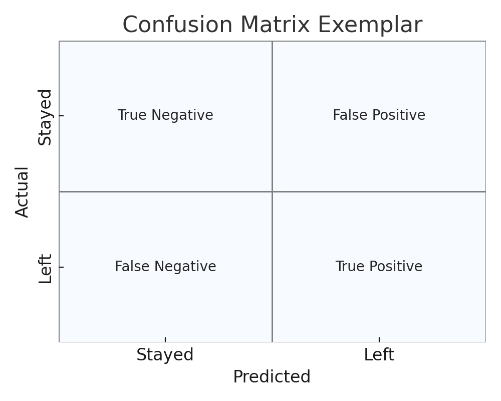
# check Variation Inflation Factor (VIF) for multicollinearity in logistic regression features
X_vif = X_train_lr.copy()
check_multicollinearity(
    X_vif,
    feature_func=None,  # no additional features for base model
    title="Correlation Matrix (base)",
)

                   feature        VIF
0       satisfaction_level   1.085652
1          last_evaluation   1.154940
2           number_project   1.253485
3    average_monthly_hours   1.178694
4                   tenure   1.126254
5            work_accident   1.004255
6    promotion_last_5years   1.015782
7                   salary   1.015677
8            department_IT   4.713044
9         department_RandD   3.772785
10   department_accounting   3.377521
11           department_hr   3.374872
12   department_management   2.600001
13    department_marketing   3.514231
14  department_product_mng   3.582268
15        department_sales  12.990657
16      department_support   8.126004
17    department_technical   9.726085


# load decision tree model and plot the tree

dt_model = joblib.load("../results/saved_models/decision_tree_(base).joblib")
estimator = dt_model.named_steps["model"]

# ensure feature_names matches columns used for training
# sklearn requires a list of strings, not a pandas index or series
feature_names = list(X_train.columns)

plt.figure(figsize=(20, 12))
plot_tree(
    estimator,
    feature_names=feature_names,
    class_names=["Stayed", "Left"],
    filled=True,
    rounded=True,
    max_depth=3,
)
plt.title("Baseline Decision Tree")
plt.tight_layout()

plt.savefig("../results/images/decision_tree_(base)_visualization.png")

plt.show()


# plot feature importance for each model

# list of model files and names
model_files = [
    ("decision_tree_(base).joblib", "Decision Tree", X_train.columns),
    ("random_forest_(base).joblib", "Random Forest", X_train.columns),
    ("xgboost_(base).joblib", "XGBoost", X_train.columns),
    ("logistic_regression_(base).joblib", "Logistic Regression", X_train_lr.columns),
]

# load each model and plot feature importance
for file_name, model_name, feature_names in model_files:
    load_and_plot_feature_importance(
        file_name, model_name, feature_names, top_n=10, save_png=True
    )


# function to add new features to the X_train / X_train_lr dataframe


# add binning features
def add_binning_features(df):
    df = df.copy()
    df["satisfaction_bin"] = pd.cut(
        df["satisfaction_level"],
        bins=[-0.01, 0.4, 0.7, 1.0],
        labels=["low", "medium", "high"],
    )
    df["hours_bin"] = pd.cut(
        df["average_monthly_hours"],
        bins=[0, 160, 240, np.inf],
        labels=["low", "medium", "high"],
    )
    df["projects_bin"] = pd.cut(
        df["number_project"], bins=[0, 2, 5, np.inf], labels=["low", "medium", "high"]
    )
    df["tenure_bin"] = pd.cut(
        df["tenure"], bins=[0, 3, 5, np.inf], labels=["short", "mid", "long"]
    )
    # encode the binned features as dummies
    df = pd.get_dummies(
        df,
        columns=["satisfaction_bin", "hours_bin", "projects_bin", "tenure_bin"],
        drop_first=True,
    )
    return df


# add interaction features
def add_interaction_features(df):
    df = df.copy()
    df["satisfaction_x_projects"] = df["satisfaction_level"] * df["number_project"]
    df["satisfaction_x_hours"] = df["satisfaction_level"] * df["average_monthly_hours"]
    df["evaluation_x_satisfaction"] = df["last_evaluation"] * df["satisfaction_level"]
    df["hours_per_project"] = df["average_monthly_hours"] / df["number_project"]
    return df


# add flag features
def add_flag_features(df):
    df = df.copy()
    df["burnout"] = (
        (df["number_project"] >= 6) | (df["average_monthly_hours"] >= 240)
    ) & (df["satisfaction_level"] <= 0.3)
    df["disengaged"] = (
        (df["number_project"] <= 2)
        & (df["average_monthly_hours"] < 160)
        & (df["satisfaction_level"] <= 0.5)
    )
    df["no_promo_4yr"] = (df["promotion_last_5years"] == 0) & (df["tenure"] >= 4)
    return df


# feature selection for logistic regression
drop_cols = [col for col in X_train_lr.columns if col.startswith("department_")]
drop_cols += ["salary", "work_accident"]
X_train_lr_fs = X_train_lr.drop(columns=drop_cols)

# feature selection for tree-based models
drop_cols = [col for col in X_train.columns if col.startswith("department_")]
drop_cols += ["salary", "work_accident"]
X_train_fs = X_train.drop(columns=drop_cols)


# logistic regression feature engineering parameters
lr_fe_params = {
    "model__C": [0.1, 1.0, 10.0],  # regularization strength (inverse)
    "model__penalty": ["l1", "l2"],  # regularization type (L1 = Lasso, L2 = Ridge)
    "model__solver": ["liblinear"],  # optimization algorithm (liblinear supports L1/L2)
    "model__class_weight": [None, "balanced"],  # None or balanced for class imbalance
}


# define feature engineered logistic regression models, their feature functions, and parameter grids
lr_fe_models = {
    "Logistic Regression with Binning": LogisticRegression(
        max_iter=1000, random_state=42
    ),
    "Logistic Regression with Interaction": LogisticRegression(
        max_iter=1000, random_state=42
    ),
    "Logistic Regression with Flags": LogisticRegression(
        max_iter=1000, random_state=42
    ),
}
lr_fe_feature_funcs = {
    "Logistic Regression with Binning": add_binning_features,
    "Logistic Regression with Interaction": add_interaction_features,
    "Logistic Regression with Flags": add_flag_features,
}
lr_fe_param_grids = {
    "Logistic Regression with Binning": lr_fe_params,
    "Logistic Regression with Interaction": lr_fe_params,
    "Logistic Regression with Flags": lr_fe_params,
}

# create models_config for logistic regression with feature engineering
lr_fe_configs = make_models_config(
    lr_fe_models,
    X_train_lr,
    y_train_lr,
    feature_func=lr_fe_feature_funcs,
    scaler=StandardScaler(),
    param_grids=lr_fe_param_grids,
)

# create models_config for logistic regression with feature engineering and feature selection
lr_fe_fs_configs = make_models_config(
    lr_fe_models,
    X_train_lr_fs,
    y_train_lr,
    feature_func=lr_fe_feature_funcs,
    scaler=StandardScaler(),
    param_grids=lr_fe_param_grids,
    name_suffix=" (Feature Selection)",
)


# run feature engineered logistic regression model evaluation
results_lr_fe_df = run_model_evaluation(
    lr_fe_configs + lr_fe_fs_configs, scoring=scoring
)
# print feature engineered model results, order by recall
print("Feature Engineered Model Evaluation Results:")
results_lr_fe_df.sort_values(by="recall", ascending=False, inplace=True)
results_lr_fe_df

Running model: Logistic Regression with Binning...
Fitting 5 folds for each of 12 candidates, totalling 60 fits
Execution time for Logistic Regression with Binning: 3.02 seconds
Best parameters for Logistic Regression with Binning: {'model__C': 0.1, 'model__class_weight': 'balanced', 'model__penalty': 'l2', 'model__solver': 'liblinear'}
Best score for Logistic Regression with Binning: 0.9375 (recall)
Model Logistic Regression with Binning not saved. Set save_model=True to save it.

Running model: Logistic Regression with Interaction...
Fitting 5 folds for each of 12 candidates, totalling 60 fits
Execution time for Logistic Regression with Interaction: 5.30 seconds
Best parameters for Logistic Regression with Interaction: {'model__C': 0.1, 'model__class_weight': 'balanced', 'model__penalty': 'l1', 'model__solver': 'liblinear'}
Best score for Logistic Regression with Interaction: 0.9336 (recall)
Model Logistic Regression with Interaction not saved. Set save_model=True to save it.

Running model: Logistic Regression with Flags...
Fitting 5 folds for each of 12 candidates, totalling 60 fits
Execution time for Logistic Regression with Flags: 1.89 seconds
Best parameters for Logistic Regression with Flags: {'model__C': 0.1, 'model__class_weight': 'balanced', 'model__penalty': 'l1', 'model__solver': 'liblinear'}
Best score for Logistic Regression with Flags: 0.9176 (recall)
Model Logistic Regression with Flags not saved. Set save_model=True to save it.

Running model: Logistic Regression with Binning (Feature Selection)...
Fitting 5 folds for each of 12 candidates, totalling 60 fits
Execution time for Logistic Regression with Binning (Feature Selection): 1.99 seconds
Best parameters for Logistic Regression with Binning (Feature Selection): {'model__C': 0.1, 'model__class_weight': 'balanced', 'model__penalty': 'l1', 'model__solver': 'liblinear'}
Best score for Logistic Regression with Binning (Feature Selection): 0.9395 (recall)
Model Logistic Regression with Binning (Feature Selection) not saved. Set save_model=True to save it.

Running model: Logistic Regression with Interaction (Feature Selection)...
Fitting 5 folds for each of 12 candidates, totalling 60 fits
Execution time for Logistic Regression with Interaction (Feature Selection): 2.67 seconds
Best parameters for Logistic Regression with Interaction (Feature Selection): {'model__C': 0.1, 'model__class_weight': 'balanced', 'model__penalty': 'l2', 'model__solver': 'liblinear'}
Best score for Logistic Regression with Interaction (Feature Selection): 0.9601 (recall)
Model Logistic Regression with Interaction (Feature Selection) not saved. Set save_model=True to save it.

Running model: Logistic Regression with Flags (Feature Selection)...
Fitting 5 folds for each of 12 candidates, totalling 60 fits
Execution time for Logistic Regression with Flags (Feature Selection): 0.81 seconds
Best parameters for Logistic Regression with Flags (Feature Selection): {'model__C': 0.1, 'model__class_weight': 'balanced', 'model__penalty': 'l1', 'model__solver': 'liblinear'}
Best score for Logistic Regression with Flags (Feature Selection): 0.9176 (recall)
Model Logistic Regression with Flags (Feature Selection) not saved. Set save_model=True to save it.

Feature Engineered Model Evaluation Results:


# plot confuision matrices for feature engineered models
plot_confusion_grid_from_results(results_lr_fe_df)
# plot_confusion_from_results(results_lr_fe_df)


# check Variation Inflation Factor (VIF) for multicollinearity
check_multicollinearity(
    X_train_lr, add_binning_features, title="Correlation Matrix with Binning"
)

                    feature        VIF
0        satisfaction_level   7.840569
1           last_evaluation   1.189989
2            number_project   2.993341
3     average_monthly_hours   6.498051
4                    tenure   3.668205
5             work_accident   1.008282
6     promotion_last_5years   1.016613
7                    salary   1.020376
8             department_IT  11.675944
9          department_RandD   8.905131
10    department_accounting   7.825115
11            department_hr   7.968615
12    department_management   5.552298
13     department_marketing   8.283252
14   department_product_mng   8.587286
15         department_sales  35.934006
16       department_support  21.514537
17     department_technical  26.238759
18  satisfaction_bin_medium   5.218627
19    satisfaction_bin_high  13.583614
20         hours_bin_medium   4.016827
21           hours_bin_high   9.224180
22      projects_bin_medium   3.149864
23        projects_bin_high   4.345744
24           tenure_bin_mid   3.898102
25          tenure_bin_long        NaN


# check Variation Inflation Factor (VIF) for multicollinearity
check_multicollinearity(
    X_train_lr, add_interaction_features, title="Correlation Matrix With Interaction"
)

                      feature        VIF
0          satisfaction_level  33.423178
1             last_evaluation  10.984233
2              number_project  15.702942
3       average_monthly_hours  14.676516
4                      tenure   1.136334
5               work_accident   1.005532
6       promotion_last_5years   1.016134
7                      salary   1.016544
8               department_IT  26.805969
9            department_RandD  20.179072
10      department_accounting  17.368028
11              department_hr  17.523350
12      department_management  11.812288
13       department_marketing  18.392598
14     department_product_mng  19.221184
15           department_sales  85.124491
16         department_support  49.944663
17       department_technical  61.178366
18    satisfaction_x_projects  19.863690
19       satisfaction_x_hours  32.334590
20  evaluation_x_satisfaction  38.731607
21          hours_per_project  10.621934


# check Variation Inflation Factor (VIF) for multicollinearity
check_multicollinearity(
    X_train_lr, add_flag_features, title="Correlation Matrix With Flags"
)

                   feature        VIF
0       satisfaction_level   1.816797
1          last_evaluation   1.207986
2           number_project   1.743925
3    average_monthly_hours   1.326410
4                   tenure   3.598575
5            work_accident   1.010532
6    promotion_last_5years   1.033890
7                   salary   1.019595
8            department_IT   8.184903
9         department_RandD   6.350736
10   department_accounting   5.586013
11           department_hr   5.666900
12   department_management   4.083762
13    department_marketing   5.907825
14  department_product_mng   6.040793
15        department_sales  24.387812
16      department_support  14.865055
17    department_technical  17.895385
18                 burnout   2.185607
19              disengaged   1.723260
20            no_promo_4yr   3.925387


# check Variation Inflation Factor (VIF) for multicollinearity
check_multicollinearity(
    X_train_lr_fs,
    add_binning_features,
    title="Correlation Matrix with Binning (Feature Selection)",
)

                    feature        VIF
0        satisfaction_level  56.543061
1           last_evaluation  21.259495
2            number_project  33.095356
3     average_monthly_hours  70.336690
4                    tenure  34.479099
5     promotion_last_5years   1.016951
6   satisfaction_bin_medium   8.429070
7     satisfaction_bin_high  23.048520
8          hours_bin_medium   5.816319
9            hours_bin_high   8.445646
10      projects_bin_medium  14.568064
11        projects_bin_high   4.688793
12           tenure_bin_mid   4.372186
13          tenure_bin_long        NaN


# check Variation Inflation Factor (VIF) for multicollinearity
check_multicollinearity(
    X_train_lr_fs,
    add_interaction_features,
    title="Correlation Matrix With Interaction (Feature Selection)",
)

                     feature         VIF
0         satisfaction_level  126.044643
1            last_evaluation  164.425397
2             number_project  154.114241
3      average_monthly_hours  261.228800
4                     tenure   14.211376
5      promotion_last_5years    1.016234
6    satisfaction_x_projects  104.982340
7       satisfaction_x_hours  160.313969
8  evaluation_x_satisfaction  166.264356
9          hours_per_project   68.161290


# check Variation Inflation Factor (VIF) for multicollinearity
check_multicollinearity(
    X_train_lr_fs,
    add_flag_features,
    title="Correlation Matrix With Flags (Feature Selection)",
)

                 feature        VIF
0     satisfaction_level  13.140748
1        last_evaluation  20.151855
2         number_project  17.576149
3  average_monthly_hours  20.522838
4                 tenure  32.730464
5  promotion_last_5years   1.032851
6                burnout   2.338252
7             disengaged   1.543493
8           no_promo_4yr   4.203340


# # tree-based feature engineering parameters
tree_fe_params = {
    "Random Forest": {
        "model__n_estimators": [100, 300],  # 300 was best, but 100 is faster for FE
        "model__max_depth": [
            3,
            4,
            5,
            8,
        ],  # 5 was best, trying for regularization, deeper trees can overfit, take longer to train
        "model__max_features": ["sqrt", 1.0],  # 1.0 was best, but sqrt is common
        "model__max_samples": [0.7, 1.0],  # 1.0 was best
        "model__min_samples_leaf": [1, 2],  # 1 or 2
        "model__min_samples_split": [2, 3],  # 2 or 3
        "model__class_weight": [
            None,
            "balanced",
        ],  # None or balanced for class imbalance
    },
    "XGBoost": {
        "model__n_estimators": [100, 300],  # 300 was best
        "model__max_depth": [
            3,
            4,
            5,
            8,
        ],  # 3 was best (moderate increase in training time)
        "model__learning_rate": [
            0.1,
            0.2,
        ],  # 0.1 is standard, 0.2 for speed, step size shrinkage
        "model__subsample": [
            0.6,
            0.8,
            1.0,
        ],  # 1.0 was best, row subsampling (adds randomness, helps generalization)
        "model__colsample_bytree": [
            0.6,
            0.8,
            1.0,
        ],  # 1.0 was best, column subsampling (adds randomness, helps generalization)
        "model__min_child_weight": [
            1,
            5,
        ],  # 1 is default, 5 for regularization, minimum sum of instance weight in a child
        "model__gamma": [
            0,
            0.1,
            0.2,
        ],  # 0.2 was best, try 0 for comparison, minimum loss reduction required to make a split
        "model__scale_pos_weight": [
            1,
            scale_pos_weight_value,
        ],  # 1 or calculated value for class imbalance
        "model__reg_alpha": [
            0,
            0.1,
            1,
        ],  # L1 regularization (helps control overfitting)
        "model__reg_lambda": [1, 2, 5],  # L2 regularization (helps control overfitting)
    },
    "Decision Tree": {
        "model__max_depth": [3, 4, 5, 6, 8],  # best was 8
        "model__min_samples_leaf": [1, 2, 3],  # 1 was best
        "model__min_samples_split": [2, 3, 4],  # 2 was best
        "model__class_weight": [
            None,
            "balanced",
        ],  # None or balanced for class imbalance
    },
}


# tree-based feature engineering configs with full model names
dt_fe_models = {
    "Decision Tree with Binning": DecisionTreeClassifier(random_state=42),
    "Decision Tree with Interaction": DecisionTreeClassifier(random_state=42),
    "Decision Tree with Flags": DecisionTreeClassifier(random_state=42),
}
rf_xgb_fe_models = {
    "Random Forest with Binning": RandomForestClassifier(random_state=42, n_jobs=-1),
    "Random Forest with Interaction": RandomForestClassifier(
        random_state=42, n_jobs=-1
    ),
    "Random Forest with Flags": RandomForestClassifier(random_state=42, n_jobs=-1),
    "XGBoost with Binning": XGBClassifier(
        eval_metric=get_xgb_eval_metric(scoring), random_state=42, n_jobs=-1
    ),
    "XGBoost with Interaction": XGBClassifier(
        eval_metric=get_xgb_eval_metric(scoring), random_state=42, n_jobs=-1
    ),
    "XGBoost with Flags": XGBClassifier(
        eval_metric=get_xgb_eval_metric(scoring), random_state=42, n_jobs=-1
    ),
}

tree_fe_feature_funcs = {
    "Random Forest with Binning": add_binning_features,
    "Random Forest with Interaction": add_interaction_features,
    "Random Forest with Flags": add_flag_features,
    "XGBoost with Binning": add_binning_features,
    "XGBoost with Interaction": add_interaction_features,
    "XGBoost with Flags": add_flag_features,
    "Decision Tree with Binning": add_binning_features,
    "Decision Tree with Interaction": add_interaction_features,
    "Decision Tree with Flags": add_flag_features,
}

tree_fe_param_grids = {
    "Random Forest with Binning": tree_fe_params["Random Forest"],
    "Random Forest with Interaction": tree_fe_params["Random Forest"],
    "Random Forest with Flags": tree_fe_params["Random Forest"],
    "XGBoost with Binning": tree_fe_params["XGBoost"],
    "XGBoost with Interaction": tree_fe_params["XGBoost"],
    "XGBoost with Flags": tree_fe_params["XGBoost"],
    "Decision Tree with Binning": tree_fe_params["Decision Tree"],
    "Decision Tree with Interaction": tree_fe_params["Decision Tree"],
    "Decision Tree with Flags": tree_fe_params["Decision Tree"],
}

# with all feature engineering functions applied
dt_fe_configs = make_models_config(
    dt_fe_models,
    X_train,
    y_train,
    feature_func=tree_fe_feature_funcs,
    param_grids=tree_fe_param_grids,
)
rf_xgb_fe_configs = make_models_config(
    rf_xgb_fe_models,
    X_train,
    y_train,
    feature_func=tree_fe_feature_funcs,
    param_grids=tree_fe_param_grids,
)

# with feature engineering and feature selection (drop_cols)
dt_fe_fs_configs = make_models_config(
    dt_fe_models,
    X_train_fs,
    y_train,
    feature_func=tree_fe_feature_funcs,
    param_grids=tree_fe_param_grids,
    name_suffix=" (feature selection)",
)
rf_xgb_fe_fs_configs = make_models_config(
    rf_xgb_fe_models,
    X_train_fs,
    y_train,
    feature_func=tree_fe_feature_funcs,
    param_grids=tree_fe_param_grids,
    name_suffix=" (feature selection)",
)


# run tree-based feature engineered model evaluation
results_tree_fe_df = run_model_evaluation(
    dt_fe_configs + dt_fe_fs_configs, scoring=scoring, search_type="grid"
)
results_tree_fe_df = run_model_evaluation(
    rf_xgb_fe_configs + rf_xgb_fe_fs_configs,
    results_df=results_tree_fe_df,
    scoring=scoring,
    search_type="random",
    n_iter=50,
)
# print feature engineered tree-based model results, order by recall
print("Feature Engineered Tree-Based Model Evaluation Results:")
results_tree_fe_df.sort_values(by="recall", ascending=False, inplace=True)
results_tree_fe_df

Running model: Decision Tree with Binning...
Fitting 5 folds for each of 90 candidates, totalling 450 fits
Execution time for Decision Tree with Binning: 5.93 seconds
Best parameters for Decision Tree with Binning: {'model__class_weight': 'balanced', 'model__max_depth': 8, 'model__min_samples_leaf': 2, 'model__min_samples_split': 2}
Best score for Decision Tree with Binning: 0.9341 (recall)
Model Decision Tree with Binning not saved. Set save_model=True to save it.

Running model: Decision Tree with Interaction...
Fitting 5 folds for each of 90 candidates, totalling 450 fits
Execution time for Decision Tree with Interaction: 6.44 seconds
Best parameters for Decision Tree with Interaction: {'model__class_weight': 'balanced', 'model__max_depth': 6, 'model__min_samples_leaf': 3, 'model__min_samples_split': 2}
Best score for Decision Tree with Interaction: 0.9334 (recall)
Model Decision Tree with Interaction not saved. Set save_model=True to save it.

Running model: Decision Tree with Flags...
Fitting 5 folds for each of 90 candidates, totalling 450 fits
Execution time for Decision Tree with Flags: 3.77 seconds
Best parameters for Decision Tree with Flags: {'model__class_weight': 'balanced', 'model__max_depth': 6, 'model__min_samples_leaf': 1, 'model__min_samples_split': 2}
Best score for Decision Tree with Flags: 0.9309 (recall)
Model Decision Tree with Flags not saved. Set save_model=True to save it.

Running model: Decision Tree with Binning (feature selection)...
Fitting 5 folds for each of 90 candidates, totalling 450 fits
Execution time for Decision Tree with Binning (feature selection): 5.51 seconds
Best parameters for Decision Tree with Binning (feature selection): {'model__class_weight': 'balanced', 'model__max_depth': 8, 'model__min_samples_leaf': 2, 'model__min_samples_split': 2}
Best score for Decision Tree with Binning (feature selection): 0.9353 (recall)
Model Decision Tree with Binning (feature selection) not saved. Set save_model=True to save it.

Running model: Decision Tree with Interaction (feature selection)...
Fitting 5 folds for each of 90 candidates, totalling 450 fits
Execution time for Decision Tree with Interaction (feature selection): 5.82 seconds
Best parameters for Decision Tree with Interaction (feature selection): {'model__class_weight': 'balanced', 'model__max_depth': 5, 'model__min_samples_leaf': 3, 'model__min_samples_split': 2}
Best score for Decision Tree with Interaction (feature selection): 0.9328 (recall)
Model Decision Tree with Interaction (feature selection) not saved. Set save_model=True to save it.

Running model: Decision Tree with Flags (feature selection)...
Fitting 5 folds for each of 90 candidates, totalling 450 fits
Execution time for Decision Tree with Flags (feature selection): 3.20 seconds
Best parameters for Decision Tree with Flags (feature selection): {'model__class_weight': 'balanced', 'model__max_depth': 6, 'model__min_samples_leaf': 1, 'model__min_samples_split': 2}
Best score for Decision Tree with Flags (feature selection): 0.9297 (recall)
Model Decision Tree with Flags (feature selection) not saved. Set save_model=True to save it.

Running model: Random Forest with Binning...
Fitting 5 folds for each of 50 candidates, totalling 250 fits
Execution time for Random Forest with Binning: 91.70 seconds
Best parameters for Random Forest with Binning: {'model__n_estimators': 300, 'model__min_samples_split': 2, 'model__min_samples_leaf': 1, 'model__max_samples': 1.0, 'model__max_features': 1.0, 'model__max_depth': 5, 'model__class_weight': 'balanced'}
Best score for Random Forest with Binning: 0.9278 (recall)
Model Random Forest with Binning not saved. Set save_model=True to save it.

Running model: Random Forest with Interaction...
Fitting 5 folds for each of 50 candidates, totalling 250 fits
Execution time for Random Forest with Interaction: 176.26 seconds
Best parameters for Random Forest with Interaction: {'model__n_estimators': 300, 'model__min_samples_split': 2, 'model__min_samples_leaf': 1, 'model__max_samples': 1.0, 'model__max_features': 1.0, 'model__max_depth': 5, 'model__class_weight': 'balanced'}
Best score for Random Forest with Interaction: 0.9297 (recall)
Model Random Forest with Interaction not saved. Set save_model=True to save it.

Running model: Random Forest with Flags...
Fitting 5 folds for each of 50 candidates, totalling 250 fits
Execution time for Random Forest with Flags: 80.66 seconds
Best parameters for Random Forest with Flags: {'model__n_estimators': 100, 'model__min_samples_split': 2, 'model__min_samples_leaf': 2, 'model__max_samples': 0.7, 'model__max_features': 1.0, 'model__max_depth': 3, 'model__class_weight': 'balanced'}
Best score for Random Forest with Flags: 0.9290 (recall)
Model Random Forest with Flags not saved. Set save_model=True to save it.

Running model: XGBoost with Binning...
Fitting 5 folds for each of 50 candidates, totalling 250 fits
Execution time for XGBoost with Binning: 24.97 seconds
Best parameters for XGBoost with Binning: {'model__subsample': 1.0, 'model__scale_pos_weight': 5.02134337727558, 'model__reg_lambda': 2, 'model__reg_alpha': 1, 'model__n_estimators': 100, 'model__min_child_weight': 5, 'model__max_depth': 3, 'model__learning_rate': 0.2, 'model__gamma': 0.1, 'model__colsample_bytree': 0.6}
Best score for XGBoost with Binning: 0.9366 (recall)
Model XGBoost with Binning not saved. Set save_model=True to save it.

Running model: XGBoost with Interaction...
Fitting 5 folds for each of 50 candidates, totalling 250 fits
Execution time for XGBoost with Interaction: 25.54 seconds
Best parameters for XGBoost with Interaction: {'model__subsample': 0.8, 'model__scale_pos_weight': 5.02134337727558, 'model__reg_lambda': 5, 'model__reg_alpha': 1, 'model__n_estimators': 100, 'model__min_child_weight': 1, 'model__max_depth': 3, 'model__learning_rate': 0.2, 'model__gamma': 0, 'model__colsample_bytree': 1.0}
Best score for XGBoost with Interaction: 0.9341 (recall)
Model XGBoost with Interaction not saved. Set save_model=True to save it.

Running model: XGBoost with Flags...
Fitting 5 folds for each of 50 candidates, totalling 250 fits
Execution time for XGBoost with Flags: 22.05 seconds
Best parameters for XGBoost with Flags: {'model__subsample': 1.0, 'model__scale_pos_weight': 5.02134337727558, 'model__reg_lambda': 2, 'model__reg_alpha': 1, 'model__n_estimators': 100, 'model__min_child_weight': 5, 'model__max_depth': 3, 'model__learning_rate': 0.2, 'model__gamma': 0.1, 'model__colsample_bytree': 0.6}
Best score for XGBoost with Flags: 0.9347 (recall)
Model XGBoost with Flags not saved. Set save_model=True to save it.

Running model: Random Forest with Binning (feature selection)...
Fitting 5 folds for each of 50 candidates, totalling 250 fits
Execution time for Random Forest with Binning (feature selection): 81.90 seconds
Best parameters for Random Forest with Binning (feature selection): {'model__n_estimators': 300, 'model__min_samples_split': 2, 'model__min_samples_leaf': 1, 'model__max_samples': 1.0, 'model__max_features': 1.0, 'model__max_depth': 5, 'model__class_weight': 'balanced'}
Best score for Random Forest with Binning (feature selection): 0.9284 (recall)
Model Random Forest with Binning (feature selection) not saved. Set save_model=True to save it.

Running model: Random Forest with Interaction (feature selection)...
Fitting 5 folds for each of 50 candidates, totalling 250 fits
Execution time for Random Forest with Interaction (feature selection): 174.32 seconds
Best parameters for Random Forest with Interaction (feature selection): {'model__n_estimators': 300, 'model__min_samples_split': 2, 'model__min_samples_leaf': 1, 'model__max_samples': 1.0, 'model__max_features': 1.0, 'model__max_depth': 5, 'model__class_weight': 'balanced'}
Best score for Random Forest with Interaction (feature selection): 0.9303 (recall)
Model Random Forest with Interaction (feature selection) not saved. Set save_model=True to save it.

Running model: Random Forest with Flags (feature selection)...
Fitting 5 folds for each of 50 candidates, totalling 250 fits
Execution time for Random Forest with Flags (feature selection): 75.86 seconds
Best parameters for Random Forest with Flags (feature selection): {'model__n_estimators': 100, 'model__min_samples_split': 2, 'model__min_samples_leaf': 2, 'model__max_samples': 0.7, 'model__max_features': 1.0, 'model__max_depth': 3, 'model__class_weight': 'balanced'}
Best score for Random Forest with Flags (feature selection): 0.9290 (recall)
Model Random Forest with Flags (feature selection) not saved. Set save_model=True to save it.

Running model: XGBoost with Binning (feature selection)...
Fitting 5 folds for each of 50 candidates, totalling 250 fits
Execution time for XGBoost with Binning (feature selection): 19.34 seconds
Best parameters for XGBoost with Binning (feature selection): {'model__subsample': 1.0, 'model__scale_pos_weight': 5.02134337727558, 'model__reg_lambda': 1, 'model__reg_alpha': 0.1, 'model__n_estimators': 100, 'model__min_child_weight': 5, 'model__max_depth': 3, 'model__learning_rate': 0.2, 'model__gamma': 0, 'model__colsample_bytree': 1.0}
Best score for XGBoost with Binning (feature selection): 0.9360 (recall)
Model XGBoost with Binning (feature selection) not saved. Set save_model=True to save it.

Running model: XGBoost with Interaction (feature selection)...
Fitting 5 folds for each of 50 candidates, totalling 250 fits
Execution time for XGBoost with Interaction (feature selection): 19.79 seconds
Best parameters for XGBoost with Interaction (feature selection): {'model__subsample': 1.0, 'model__scale_pos_weight': 5.02134337727558, 'model__reg_lambda': 1, 'model__reg_alpha': 0.1, 'model__n_estimators': 100, 'model__min_child_weight': 5, 'model__max_depth': 3, 'model__learning_rate': 0.2, 'model__gamma': 0, 'model__colsample_bytree': 1.0}
Best score for XGBoost with Interaction (feature selection): 0.9316 (recall)
Model XGBoost with Interaction (feature selection) not saved. Set save_model=True to save it.

Running model: XGBoost with Flags (feature selection)...
Fitting 5 folds for each of 50 candidates, totalling 250 fits
Execution time for XGBoost with Flags (feature selection): 15.63 seconds
Best parameters for XGBoost with Flags (feature selection): {'model__subsample': 1.0, 'model__scale_pos_weight': 5.02134337727558, 'model__reg_lambda': 5, 'model__reg_alpha': 1, 'model__n_estimators': 300, 'model__min_child_weight': 5, 'model__max_depth': 3, 'model__learning_rate': 0.1, 'model__gamma': 0, 'model__colsample_bytree': 1.0}
Best score for XGBoost with Flags (feature selection): 0.9353 (recall)
Model XGBoost with Flags (feature selection) not saved. Set save_model=True to save it.

Feature Engineered Tree-Based Model Evaluation Results:


# selected features + burnout flag
def select_core_features_with_burnout(df):
    df = df.copy()
    # burnout flag: (projects >= 6 or hours >= 240) & satisfaction <= 0.3
    df["burnout"] = (
        (df["number_project"] >= 6) | (df["average_monthly_hours"] >= 240)
    ) & (df["satisfaction_level"] <= 0.3)
    return df[
        [
            "satisfaction_level",
            "last_evaluation",
            "number_project",
            "average_monthly_hours",
            "tenure",
            "promotion_last_5years",
            "burnout",
        ]
    ]


# selected features + interactions
def select_core_features_with_interactions(df):
    df = df.copy()
    # interactions
    df["satisfaction_x_projects"] = df["satisfaction_level"] * df["number_project"]
    df["hours_per_project"] = df["average_monthly_hours"] / df["number_project"]
    return df[
        [
            "satisfaction_level",
            "number_project",
            "average_monthly_hours",
            "tenure",
            "satisfaction_x_projects",
            "hours_per_project",
        ]
    ]


# selected features + interactions + burnout flag
def select_core_features_with_interactions_and_burnout(df):
    df = df.copy()
    # burnout flag: (projects >= 6 or hours >= 240) & satisfaction <= 0.3
    df["burnout"] = (
        (df["number_project"] >= 6) | (df["average_monthly_hours"] >= 240)
    ) & (df["satisfaction_level"] <= 0.3)
    # interaction
    df["satisfaction_x_projects"] = df["satisfaction_level"] * df["number_project"]
    return df[
        [
            "satisfaction_level",
            "number_project",
            "average_monthly_hours",
            "tenure",
            "burnout",
            "satisfaction_x_projects",
        ]
    ]


# --- Feature engineering round 2 model dicts ---

# logistic regression FE2 models, feature funcs, param grids
lr_fe2_models = {
    "Logistic Regression (Core + Burnout)": LogisticRegression(
        max_iter=1000, random_state=42
    ),
    "Logistic Regression (Core + Interactions)": LogisticRegression(
        max_iter=1000, random_state=42
    ),
    "Logistic Regression (Core + Interactions + Burnout)": LogisticRegression(
        max_iter=1000, random_state=42
    ),
}
lr_fe2_feature_funcs = {
    "Logistic Regression (Core + Burnout)": select_core_features_with_burnout,
    "Logistic Regression (Core + Interactions)": select_core_features_with_interactions,
    "Logistic Regression (Core + Interactions + Burnout)": select_core_features_with_interactions_and_burnout,
}
lr_fe2_param_grids = {
    "Logistic Regression (Core + Burnout)": lr_fe_params,
    "Logistic Regression (Core + Interactions)": lr_fe_params,
    "Logistic Regression (Core + Interactions + Burnout)": lr_fe_params,
}

# tree-based FE2 models, feature funcs, param grids
dt_fe2_models = {
    "Decision Tree (Core + Burnout)": DecisionTreeClassifier(random_state=42),
    "Decision Tree (Core + Interactions)": DecisionTreeClassifier(random_state=42),
    "Decision Tree (Core + Interactions + Burnout)": DecisionTreeClassifier(
        random_state=42
    ),
}
rf_xgb_fe2_models = {
    "Random Forest (Core + Burnout)": RandomForestClassifier(
        random_state=42, n_jobs=-1
    ),
    "Random Forest (Core + Interactions)": RandomForestClassifier(
        random_state=42, n_jobs=-1
    ),
    "Random Forest (Core + Interactions + Burnout)": RandomForestClassifier(
        random_state=42, n_jobs=-1
    ),
    "XGBoost (Core + Burnout)": XGBClassifier(
        eval_metric=get_xgb_eval_metric(scoring), random_state=42, n_jobs=-1
    ),
    "XGBoost (Core + Interactions)": XGBClassifier(
        eval_metric=get_xgb_eval_metric(scoring), random_state=42, n_jobs=-1
    ),
    "XGBoost (Core + Interactions + Burnout)": XGBClassifier(
        eval_metric=get_xgb_eval_metric(scoring), random_state=42, n_jobs=-1
    ),
}
tree_fe2_feature_funcs = {
    "Decision Tree (Core + Burnout)": select_core_features_with_burnout,
    "Decision Tree (Core + Interactions)": select_core_features_with_interactions,
    "Decision Tree (Core + Interactions + Burnout)": select_core_features_with_interactions_and_burnout,
    "Random Forest (Core + Burnout)": select_core_features_with_burnout,
    "Random Forest (Core + Interactions)": select_core_features_with_interactions,
    "Random Forest (Core + Interactions + Burnout)": select_core_features_with_interactions_and_burnout,
    "XGBoost (Core + Burnout)": select_core_features_with_burnout,
    "XGBoost (Core + Interactions)": select_core_features_with_interactions,
    "XGBoost (Core + Interactions + Burnout)": select_core_features_with_interactions_and_burnout,
}
tree_fe2_param_grids = {
    "Decision Tree (Core + Burnout)": tree_fe_params["Decision Tree"],
    "Decision Tree (Core + Interactions)": tree_fe_params["Decision Tree"],
    "Decision Tree (Core + Interactions + Burnout)": tree_fe_params["Decision Tree"],
    "Random Forest (Core + Burnout)": tree_fe_params["Random Forest"],
    "Random Forest (Core + Interactions)": tree_fe_params["Random Forest"],
    "Random Forest (Core + Interactions + Burnout)": tree_fe_params["Random Forest"],
    "XGBoost (Core + Burnout)": tree_fe_params["XGBoost"],
    "XGBoost (Core + Interactions)": tree_fe_params["XGBoost"],
    "XGBoost (Core + Interactions + Burnout)": tree_fe_params["XGBoost"],
}

# create models_config for FE2 models
lr_fe2_configs = make_models_config(
    lr_fe2_models,
    X_train_lr,
    y_train_lr,
    feature_func=lr_fe2_feature_funcs,
    scaler=StandardScaler(),
    param_grids=lr_fe2_param_grids,
)
dt_fe2_configs = make_models_config(
    dt_fe2_models,
    X_train,
    y_train,
    feature_func=tree_fe2_feature_funcs,
    param_grids=tree_fe2_param_grids,
)
rf_xgb_fe2_configs = make_models_config(
    rf_xgb_fe2_models,
    X_train,
    y_train,
    feature_func=tree_fe2_feature_funcs,
    param_grids=tree_fe2_param_grids,
)


# run feature engineered round 2 model evaluation
results_fe2_df = run_model_evaluation(
    lr_fe2_configs, scoring=scoring, search_type="grid"
)
results_fe2_df = run_model_evaluation(
    dt_fe2_configs, results_df=results_fe2_df, scoring=scoring, search_type="grid"
)
results_fe2_df = run_model_evaluation(
    rf_xgb_fe2_configs,
    results_df=results_fe2_df,
    scoring=scoring,
    search_type="random",
    n_iter=50,
)
# print feature engineered round 2 model results, order by recall
print("Feature Engineered Round 2 Model Evaluation Results:")
results_fe2_df.sort_values(by="recall", ascending=False, inplace=True)
results_fe2_df

Running model: Logistic Regression (Core + Burnout)...
Fitting 5 folds for each of 12 candidates, totalling 60 fits
Execution time for Logistic Regression (Core + Burnout): 0.55 seconds
Best parameters for Logistic Regression (Core + Burnout): {'model__C': 0.1, 'model__class_weight': 'balanced', 'model__penalty': 'l1', 'model__solver': 'liblinear'}
Best score for Logistic Regression (Core + Burnout): 0.9349 (recall)
Model Logistic Regression (Core + Burnout) not saved. Set save_model=True to save it.

Running model: Logistic Regression (Core + Interactions)...
Fitting 5 folds for each of 12 candidates, totalling 60 fits
Execution time for Logistic Regression (Core + Interactions): 0.75 seconds
Best parameters for Logistic Regression (Core + Interactions): {'model__C': 0.1, 'model__class_weight': 'balanced', 'model__penalty': 'l1', 'model__solver': 'liblinear'}
Best score for Logistic Regression (Core + Interactions): 0.9621 (recall)
Model Logistic Regression (Core + Interactions) not saved. Set save_model=True to save it.

Running model: Logistic Regression (Core + Interactions + Burnout)...
Fitting 5 folds for each of 12 candidates, totalling 60 fits
Execution time for Logistic Regression (Core + Interactions + Burnout): 0.89 seconds
Best parameters for Logistic Regression (Core + Interactions + Burnout): {'model__C': 0.1, 'model__class_weight': 'balanced', 'model__penalty': 'l2', 'model__solver': 'liblinear'}
Best score for Logistic Regression (Core + Interactions + Burnout): 0.9515 (recall)
Model Logistic Regression (Core + Interactions + Burnout) not saved. Set save_model=True to save it.

Running model: Decision Tree (Core + Burnout)...
Fitting 5 folds for each of 90 candidates, totalling 450 fits
Execution time for Decision Tree (Core + Burnout): 3.43 seconds
Best parameters for Decision Tree (Core + Burnout): {'model__class_weight': 'balanced', 'model__max_depth': 5, 'model__min_samples_leaf': 1, 'model__min_samples_split': 2}
Best score for Decision Tree (Core + Burnout): 0.9435 (recall)
Model Decision Tree (Core + Burnout) not saved. Set save_model=True to save it.

Running model: Decision Tree (Core + Interactions)...
Fitting 5 folds for each of 90 candidates, totalling 450 fits
Execution time for Decision Tree (Core + Interactions): 4.01 seconds
Best parameters for Decision Tree (Core + Interactions): {'model__class_weight': 'balanced', 'model__max_depth': 8, 'model__min_samples_leaf': 3, 'model__min_samples_split': 2}
Best score for Decision Tree (Core + Interactions): 0.9316 (recall)
Model Decision Tree (Core + Interactions) not saved. Set save_model=True to save it.

Running model: Decision Tree (Core + Interactions + Burnout)...
Fitting 5 folds for each of 90 candidates, totalling 450 fits
Execution time for Decision Tree (Core + Interactions + Burnout): 3.67 seconds
Best parameters for Decision Tree (Core + Interactions + Burnout): {'model__class_weight': 'balanced', 'model__max_depth': 5, 'model__min_samples_leaf': 1, 'model__min_samples_split': 2}
Best score for Decision Tree (Core + Interactions + Burnout): 0.9303 (recall)
Model Decision Tree (Core + Interactions + Burnout) not saved. Set save_model=True to save it.

Running model: Random Forest (Core + Burnout)...
Fitting 5 folds for each of 50 candidates, totalling 250 fits
Execution time for Random Forest (Core + Burnout): 71.97 seconds
Best parameters for Random Forest (Core + Burnout): {'model__n_estimators': 300, 'model__min_samples_split': 2, 'model__min_samples_leaf': 1, 'model__max_samples': 1.0, 'model__max_features': 1.0, 'model__max_depth': 5, 'model__class_weight': 'balanced'}
Best score for Random Forest (Core + Burnout): 0.9410 (recall)
Model Random Forest (Core + Burnout) not saved. Set save_model=True to save it.

Running model: Random Forest (Core + Interactions)...
Fitting 5 folds for each of 50 candidates, totalling 250 fits
Execution time for Random Forest (Core + Interactions): 93.47 seconds
Best parameters for Random Forest (Core + Interactions): {'model__n_estimators': 100, 'model__min_samples_split': 2, 'model__min_samples_leaf': 1, 'model__max_samples': 1.0, 'model__max_features': 1.0, 'model__max_depth': 3, 'model__class_weight': 'balanced'}
Best score for Random Forest (Core + Interactions): 0.9278 (recall)
Model Random Forest (Core + Interactions) not saved. Set save_model=True to save it.

Running model: Random Forest (Core + Interactions + Burnout)...
Fitting 5 folds for each of 50 candidates, totalling 250 fits
Execution time for Random Forest (Core + Interactions + Burnout): 79.04 seconds
Best parameters for Random Forest (Core + Interactions + Burnout): {'model__n_estimators': 100, 'model__min_samples_split': 3, 'model__min_samples_leaf': 2, 'model__max_samples': 1.0, 'model__max_features': 1.0, 'model__max_depth': 5, 'model__class_weight': 'balanced'}
Best score for Random Forest (Core + Interactions + Burnout): 0.9297 (recall)
Model Random Forest (Core + Interactions + Burnout) not saved. Set save_model=True to save it.

Running model: XGBoost (Core + Burnout)...
Fitting 5 folds for each of 50 candidates, totalling 250 fits
Execution time for XGBoost (Core + Burnout): 14.96 seconds
Best parameters for XGBoost (Core + Burnout): {'model__subsample': 1.0, 'model__scale_pos_weight': 5.02134337727558, 'model__reg_lambda': 2, 'model__reg_alpha': 1, 'model__n_estimators': 100, 'model__min_child_weight': 5, 'model__max_depth': 3, 'model__learning_rate': 0.2, 'model__gamma': 0.1, 'model__colsample_bytree': 0.6}
Best score for XGBoost (Core + Burnout): 0.9366 (recall)
Model XGBoost (Core + Burnout) not saved. Set save_model=True to save it.

Running model: XGBoost (Core + Interactions)...
Fitting 5 folds for each of 50 candidates, totalling 250 fits
Execution time for XGBoost (Core + Interactions): 15.85 seconds
Best parameters for XGBoost (Core + Interactions): {'model__subsample': 1.0, 'model__scale_pos_weight': 5.02134337727558, 'model__reg_lambda': 2, 'model__reg_alpha': 1, 'model__n_estimators': 100, 'model__min_child_weight': 5, 'model__max_depth': 3, 'model__learning_rate': 0.2, 'model__gamma': 0.1, 'model__colsample_bytree': 0.6}
Best score for XGBoost (Core + Interactions): 0.9309 (recall)
Model XGBoost (Core + Interactions) not saved. Set save_model=True to save it.

Running model: XGBoost (Core + Interactions + Burnout)...
Fitting 5 folds for each of 50 candidates, totalling 250 fits
Execution time for XGBoost (Core + Interactions + Burnout): 15.30 seconds
Best parameters for XGBoost (Core + Interactions + Burnout): {'model__subsample': 1.0, 'model__scale_pos_weight': 5.02134337727558, 'model__reg_lambda': 2, 'model__reg_alpha': 1, 'model__n_estimators': 100, 'model__min_child_weight': 5, 'model__max_depth': 3, 'model__learning_rate': 0.2, 'model__gamma': 0.1, 'model__colsample_bytree': 0.6}
Best score for XGBoost (Core + Interactions + Burnout): 0.9322 (recall)
Model XGBoost (Core + Interactions + Burnout) not saved. Set save_model=True to save it.

Feature Engineered Round 2 Model Evaluation Results:


# plot confusion matrices for feature engineered round 2 models
plot_confusion_grid_from_results(results_fe2_df)
# plot_confusion_from_results(results_fe2_df)


# function to add NEW AND IMPROVVED MULTICOLLINEARITY-CORRECTIVE features to the X_train / X_train_lr dataframe
# in an unsurprising twist, it won't work


# add binning features
def add_binning_features_minimal(df):
    df = df.copy()
    df["satisfaction_bin"] = pd.cut(
        df["satisfaction_level"],
        bins=[-0.01, 0.4, 0.7, 1.0],
        labels=["low", "medium", "high"],
    )
    df["hours_bin"] = pd.cut(
        df["average_monthly_hours"],
        bins=[0, 160, 240, np.inf],
        labels=["low", "medium", "high"],
    )
    df["projects_bin"] = pd.cut(
        df["number_project"], bins=[0, 2, 5, np.inf], labels=["low", "medium", "high"]
    )
    df["tenure_bin"] = pd.cut(
        df["tenure"], bins=[0, 3, 5, np.inf], labels=["short", "mid", "long"]
    )
    # encode the binned features as dummies
    df = pd.get_dummies(
        df,
        columns=["satisfaction_bin", "hours_bin", "projects_bin", "tenure_bin"],
        drop_first=True,
    )
    # drop original columns that were binned to reduce multicollinearity
    drop_cols = [col for col in X_train_lr.columns if col.startswith("department_")]
    drop_cols += [
        "salary",
        "work_accident",
        "satisfaction_level",
        "average_monthly_hours",
        "number_project",
        "tenure",
        "last_evaluation",
    ]
    df = df.drop(columns=drop_cols)
    return df


# add interaction features
def add_interaction_features_minimal(df):
    df = df.copy()
    # Create interaction features
    df["satisfaction_x_projects"] = df["satisfaction_level"] * df["number_project"]
    df["satisfaction_x_hours"] = df["satisfaction_level"] * df["average_monthly_hours"]
    df["evaluation_x_satisfaction"] = df["last_evaluation"] * df["satisfaction_level"]
    df["hours_per_project"] = df["average_monthly_hours"] / df["number_project"]
    # drop the original columns to reduce multicollinearity
    drop_cols = [col for col in X_train_lr.columns if col.startswith("department_")]
    drop_cols += [
        "salary",
        "work_accident",
        "satisfaction_level",
        "average_monthly_hours",
        "number_project",
        "last_evaluation",
    ]
    df = df.drop(columns=drop_cols)
    return df


# check Variation Inflation Factor (VIF) for multicollinearity
check_multicollinearity(
    X_train_lr,
    add_binning_features_minimal,
    title="Correlation Matrix (Minimal Binned)",
)

                   feature       VIF
0    promotion_last_5years  1.016357
1  satisfaction_bin_medium  2.722151
2    satisfaction_bin_high  3.688523
3         hours_bin_medium  2.936013
4           hours_bin_high  2.224566
5      projects_bin_medium  6.793247
6        projects_bin_high  1.593423
7           tenure_bin_mid  1.589150
8          tenure_bin_long       NaN


# check Variation Inflation Factor (VIF) for multicollinearity
check_multicollinearity(
    X_train_lr,
    add_interaction_features_minimal,
    title="Correlation Matrix (Minimal Interaction)",
)

                     feature        VIF
0                     tenure   9.666223
1      promotion_last_5years   1.016154
2    satisfaction_x_projects  26.015651
3       satisfaction_x_hours  33.423064
4  evaluation_x_satisfaction  16.542508
5          hours_per_project  14.624745


# check Variation Inflation Factor (VIF) for multicollinearity
check_multicollinearity(
    X_train_lr,
    select_core_features_with_burnout,
    title="Correlation Matrix (Core + Burnout)",
)

                 feature        VIF
0     satisfaction_level  12.306949
1        last_evaluation  19.607589
2         number_project  16.269323
3  average_monthly_hours  19.603523
4                 tenure  11.795459
5  promotion_last_5years   1.016235
6                burnout   2.267190


# check Variation Inflation Factor (VIF) for multicollinearity
check_multicollinearity(
    X_train_lr,
    select_core_features_with_interactions,
    title="Correlation Matrix (Core + Interactions)",
)

                   feature        VIF
0       satisfaction_level  75.925035
1           number_project  35.708212
2    average_monthly_hours  68.737886
3                   tenure  13.937786
4  satisfaction_x_projects  65.715553
5        hours_per_project  47.675685


# check Variation Inflation Factor (VIF) for multicollinearity
check_multicollinearity(
    X_train_lr,
    select_core_features_with_interactions_and_burnout,
    title="Correlation Matrix (Core + Interactions + Burnout)",
)

                   feature        VIF
0       satisfaction_level  37.877753
1           number_project  38.482778
2    average_monthly_hours  21.647122
3                   tenure  12.873584
4                  burnout   2.514151
5  satisfaction_x_projects  42.220187


# # refresher
# # logistic regression feature engineering parameters
# lr_fe_params = {
#     "model__C": [0.1, 1.0, 10.0],  # regularization strength (inverse)
#     "model__penalty": ["l1", "l2"],  # regularization type (L1 = Lasso, L2 = Ridge)
#     "model__solver": ["liblinear"],  # optimization algorithm (liblinear supports L1/L2)
#     "model__class_weight": [None, "balanced"],  # None or balanced for class imbalance
# }


def drop_minimal_features(df):
    """
    Drops department dummies, salary, and work_accident columns from the input DataFrame.
    Returns a new DataFrame with those columns removed.
    """
    drop_cols = [col for col in df.columns if col.startswith("department_")]
    drop_cols += ["salary", "work_accident"]
    return df.drop(columns=drop_cols)


# check Variation Inflation Factor (VIF) for multicollinearity
check_multicollinearity(
    X_train_lr, drop_minimal_features, title="Correlation Matrix (Minimal Base)"
)

                 feature        VIF
0     satisfaction_level   6.916792
1        last_evaluation  19.597350
2         number_project  14.041656
3  average_monthly_hours  18.508819
4                 tenure  11.793165
5  promotion_last_5years   1.015986


# define feature engineered logistic regression models, their feature functions, and parameter grids
lr_minimal_models = {
    "Logistic Regression (Minimal Binned)": LogisticRegression(
        max_iter=1000, random_state=42
    ),
    "Logistic Regression (Minimal Interaction)": LogisticRegression(
        max_iter=1000, random_state=42
    ),
    "Logistic Regression (Minimal Base)": LogisticRegression(
        max_iter=1000, random_state=42
    ),
}
lr_minimal_feature_funcs = {
    "Logistic Regression (Minimal Binned)": add_binning_features_minimal,
    "Logistic Regression (Minimal Interaction)": add_interaction_features_minimal,
    "Logistic Regression (Minimal Base)": drop_minimal_features,
}
lr_minimal_param_grids = {
    "Logistic Regression (Minimal Binned)": lr_fe_params,
    "Logistic Regression (Minimal Interaction)": lr_fe_params,
    "Logistic Regression (Minimal Base)": lr_fe_params,
}

# create models_config for logistic regression with feature engineering
lr_minimal_configs = make_models_config(
    lr_minimal_models,
    X_train_lr,
    y_train_lr,
    feature_func=lr_minimal_feature_funcs,
    scaler=StandardScaler(),
    param_grids=lr_minimal_param_grids,
)


# run minimal feature engineered logistic regression model evaluation
results_lr_minimal_df = run_model_evaluation(lr_minimal_configs, scoring=scoring)
# print feature engineered model results, order by recall
print("Minimal Feature Engineered Model Evaluation Results:")
results_lr_minimal_df.sort_values(by="recall", ascending=False, inplace=True)
results_lr_minimal_df

Running model: Logistic Regression (Minimal Binned)...
Fitting 5 folds for each of 12 candidates, totalling 60 fits
Execution time for Logistic Regression (Minimal Binned): 0.81 seconds
Best parameters for Logistic Regression (Minimal Binned): {'model__C': 0.1, 'model__class_weight': 'balanced', 'model__penalty': 'l1', 'model__solver': 'liblinear'}
Best score for Logistic Regression (Minimal Binned): 0.8784 (recall)
Model Logistic Regression (Minimal Binned) not saved. Set save_model=True to save it.

Running model: Logistic Regression (Minimal Interaction)...
Fitting 5 folds for each of 12 candidates, totalling 60 fits
Execution time for Logistic Regression (Minimal Interaction): 0.66 seconds
Best parameters for Logistic Regression (Minimal Interaction): {'model__C': 10.0, 'model__class_weight': 'balanced', 'model__penalty': 'l1', 'model__solver': 'liblinear'}
Best score for Logistic Regression (Minimal Interaction): 0.9409 (recall)
Model Logistic Regression (Minimal Interaction) not saved. Set save_model=True to save it.

Running model: Logistic Regression (Minimal Base)...
Fitting 5 folds for each of 12 candidates, totalling 60 fits
Execution time for Logistic Regression (Minimal Base): 0.42 seconds
Best parameters for Logistic Regression (Minimal Base): {'model__C': 0.1, 'model__class_weight': 'balanced', 'model__penalty': 'l2', 'model__solver': 'liblinear'}
Best score for Logistic Regression (Minimal Base): 0.9442 (recall)
Model Logistic Regression (Minimal Base) not saved. Set save_model=True to save it.

Minimal Feature Engineered Model Evaluation Results:


# plot confuision matrices for minimal feature engineered models
plot_confusion_grid_from_results(results_lr_minimal_df)
# plot_confusion_from_results(results_lr_minimal_df)


# merge all results dataframes into a single dataframe for comparison
all_results_df = pd.concat(
    [
        results_df,
        results_lr_fe_df,
        results_tree_fe_df,
        results_fe2_df,
        results_lr_minimal_df,
    ],
    ignore_index=True,
)
all_results_df.sort_values(by="recall", ascending=False, inplace=True)
print("All Model Evaluation Results:")
all_results_df

All Model Evaluation Results:


# save results to CSV
results_df.to_csv("../results/base_model_evaluation_results.csv", index=False)
results_lr_fe_df.to_csv(
    "../results/logistic_regression_feature_engineered_results.csv", index=False
)
results_tree_fe_df.to_csv(
    "../results/tree_based_feature_engineered_results.csv", index=False
)
results_fe2_df.to_csv("../results/feature_engineered_round_2_results.csv", index=False)
results_lr_minimal_df.to_csv(
    "../results/logistic_regression_minimal_feature_engineered_results.csv", index=False
)
all_results_df.to_csv("../results/all_model_evaluation_results.csv", index=False)


# plot confusion matrices for all models in a grid
plot_confusion_grid_from_results(all_results_df)


plot_confusion_grid_from_results(
    all_results_df.iloc[:9], png_title="Top Model Confusion Matrices"
)


# print all_results_df, ordered by alternate metrics
metrics = ["f2", "f1", "accuracy", "roc_auc", "precision", "pr_auc"]

for metric in metrics:
    print(f"\n\n\n--- Sorted by {metric} (descending) ---")
    display(all_results_df.sort_values(by=metric, ascending=False))



--- Sorted by f2 (descending) ---



--- Sorted by f1 (descending) ---



--- Sorted by accuracy (descending) ---



--- Sorted by roc_auc (descending) ---



--- Sorted by precision (descending) ---



--- Sorted by pr_auc (descending) ---


# print total execution time, for measuring performance
nb_end_time = time.time()
print(f"Total execution time: {nb_end_time - nb_start_time:.2f} seconds")
print(
    f"Total execution time: {time.strftime('%H:%M:%S', time.gmtime(nb_end_time - nb_start_time))}"
)

Total execution time: 1591.96 seconds
Total execution time: 00:26:31

Variable	Description
satisfaction_level	Employee-reported job satisfaction level [0–1]
last_evaluation	Score of employee's last performance review [0–1]
number_project	Number of projects employee contributes to
average_monthly_hours	Average number of hours employee worked per month
time_spend_company	How long the employee has been with the company (years)
Work_accident	Whether or not the employee experienced an accident while at work
left	Whether or not the employee left the company
promotion_last_5years	Whether or not the employee was promoted in the last 5 years
Department	The employee's department
salary	The employee's salary (U.S. dollars)

Variable	Description
Bins
satisfaction_bin_low	Binary indicator: satisfaction_level is low (≤ 0.4)
satisfaction_bin_medium	Binary indicator: satisfaction_level is medium (> 0.4 and ≤ 0.7)
satisfaction_bin_high	Binary indicator: satisfaction_level is high (> 0.7)
hours_bin_low	Binary indicator: average_monthly_hours is low (≤ 160)
hours_bin_medium	Binary indicator: average_monthly_hours is medium (> 160 and ≤ 240)
hours_bin_high	Binary indicator: average_monthly_hours is high (> 240)
projects_bin_low	Binary indicator: number_project is low (≤ 2)
projects_bin_medium	Binary indicator: number_project is medium (> 2 and ≤ 5)
projects_bin_high	Binary indicator: number_project is high (> 5)
tenure_bin_short	Binary indicator: tenure is short (≤ 3 years)
tenure_bin_mid	Binary indicator: tenure is mid (> 3 and ≤ 5 years)
tenure_bin_long	Binary indicator: tenure is long (> 5 years)
Interactions
satisfaction_x_projects	Interaction: satisfaction_level × number_project
satisfaction_x_hours	Interaction: satisfaction_level × average_monthly_hours
evaluation_x_satisfaction	Interaction: last_evaluation × satisfaction_level
hours_per_project	Ratio: average_monthly_hours divided by number_project
Flags
burnout	Flag: True if (number_project ≥ 6 or average_monthly_hours ≥ 240) and satisfaction_level ≤ 0.3
disengaged	Flag: True if (number_project ≤ 2 and average_monthly_hours < 160 and satisfaction_level ≤ 0.5)
no_promo_4yr	Flag: True if promotion_last_5years == 0 and tenure ≥ 4

	satisfaction_level	last_evaluation	number_project	average_montly_hours	time_spend_company	Work_accident	left	promotion_last_5years
count	14999.000000	14999.000000	14999.000000	14999.000000	14999.000000	14999.000000	14999.000000	14999.000000
mean	0.612834	0.716102	3.803054	201.050337	3.498233	0.144610	0.238083	0.021268
std	0.248631	0.171169	1.232592	49.943099	1.460136	0.351719	0.425924	0.144281
min	0.090000	0.360000	2.000000	96.000000	2.000000	0.000000	0.000000	0.000000
25%	0.440000	0.560000	3.000000	156.000000	3.000000	0.000000	0.000000	0.000000
50%	0.640000	0.720000	4.000000	200.000000	3.000000	0.000000	0.000000	0.000000
75%	0.820000	0.870000	5.000000	245.000000	4.000000	0.000000	0.000000	0.000000
max	1.000000	1.000000	7.000000	310.000000	10.000000	1.000000	1.000000	1.000000

Item	number_project	left	Count	Percent
0	2	Left	857.0	54.17
1	2	Stayed	725.0	45.83
2	3	Left	38.0	1.08
3	3	Stayed	3482.0	98.92
4	4	Left	237.0	6.43
5	4	Stayed	3448.0	93.57
6	5	Left	343.0	15.36
7	5	Stayed	1890.0	84.64
8	6	Left	371.0	44.92
9	6	Stayed	455.0	55.08
10	7	Left	145.0	100.00
11	7	Stayed	0.0	0.00

	model	recall	f2	f1	pr_auc	roc_auc	precision	accuracy	features	best_params	cv_best_score	conf_matrix	search_time
0	Logistic Regression (base)	0.947508	0.796203	0.642342	0.464504	0.891388	0.485860	0.822232	18	{'model__C': 0.01, 'model__class_weight': 'bal...	0.947508	[[5919, 1509], [79, 1426]]	5.255588
1	Decision Tree (base)	0.942247	0.881179	0.803103	0.751529	0.945551	0.699767	0.923269	18	{'model__class_weight': 'balanced', 'model__ma...	0.942243	[[7355, 644], [92, 1501]]	3.081794
2	Random Forest (base)	0.940364	0.863799	0.769784	0.846457	0.964169	0.651588	0.906589	18	{'model__n_estimators': 500, 'model__min_sampl...	0.940354	[[7198, 801], [95, 1498]]	198.148717
3	XGBoost (base)	0.936598	0.926018	0.910589	0.967351	0.986294	0.885986	0.969454	18	{'model__subsample': 1.0, 'model__scale_pos_we...	0.936592	[[7807, 192], [101, 1492]]	20.325400

	satisfaction_level	last_evaluation	number_project	average_montly_hours	time_spend_company	left	Department	salary
0	0.38	0.53	2	157	3	1	sales	low
1	0.80	0.86	5	262	6	1	sales	medium
2	0.11	0.88	7	272	4	1	sales	medium
3	0.72	0.87	5	223	5	1	sales	low
4	0.37	0.52	2	159	3	1	sales	low

	satisfaction_level	last_evaluation	number_project	average_monthly_hours	tenure	left	department	salary
396	0.46	0.57	2	139	3	1	sales	low
866	0.41	0.46	2	128	3	1	accounting	low
1317	0.37	0.51	2	127	3	1	sales	medium
1368	0.41	0.52	2	132	3	1	RandD	low
1461	0.42	0.53	2	142	3	1	sales	low

	Tenure	Left	Count	Percent
0	2	Stayed	2879	98.934708
1	2	Left	31	1.065292
2	3	Stayed	4316	83.159923
3	3	Left	874	16.840077
4	4	Stayed	1510	75.311721
5	4	Left	495	24.688279
6	5	Stayed	580	54.613936
7	5	Left	482	45.386064
8	6	Stayed	433	79.889299
9	6	Left	109	20.110701
10	7	Stayed	94	100.000000
11	7	Left	0	0.000000
12	8	Stayed	81	100.000000
13	8	Left	0	0.000000
14	10	Stayed	107	100.000000
15	10	Left	0	0.000000

Item	department	Left	Count	Percent
0	IT	Left	158.0	16.19
1	IT	Stayed	818.0	83.81
2	RandD	Left	85.0	12.25
3	RandD	Stayed	609.0	87.75
4	accounting	Left	109.0	17.55
5	accounting	Stayed	512.0	82.45
6	hr	Left	113.0	18.80
7	hr	Stayed	488.0	81.20
8	management	Left	52.0	11.93
9	management	Stayed	384.0	88.07
10	marketing	Left	112.0	16.64
11	marketing	Stayed	561.0	83.36
12	product_mng	Left	110.0	16.03
13	product_mng	Stayed	576.0	83.97
14	sales	Left	550.0	16.98
15	sales	Stayed	2689.0	83.02
16	support	Left	312.0	17.13
17	support	Stayed	1509.0	82.87
18	technical	Left	390.0	17.38
19	technical	Stayed	1854.0	82.62

Item	salary	Left	Count	Percent
0	high	Left	48.0	4.85
1	high	Stayed	942.0	95.15
2	low	Left	1174.0	20.45
3	low	Stayed	4566.0	79.55
4	medium	Left	769.0	14.62
5	medium	Stayed	4492.0	85.38

Item	work_accident	left	Count	Percent
0	No	Left	1886.0	18.60
1	No	Stayed	8255.0	81.40
2	Yes	Left	105.0	5.68
3	Yes	Stayed	1745.0	94.32

	model	recall	f2	f1	pr_auc	roc_auc	precision	accuracy	features	best_params	cv_best_score	conf_matrix	search_time
4	Logistic Regression with Interaction (Feature ...	0.960133	0.819161	0.671312	0.452351	0.891666	0.516071	0.841599	10	{'model__C': 0.1, 'model__class_weight': 'bala...	0.960133	[[6073, 1355], [60, 1445]]	2.670381
3	Logistic Regression with Binning (Feature Sele...	0.939535	0.855104	0.753531	0.708096	0.947481	0.629004	0.896451	14	{'model__C': 0.1, 'model__class_weight': 'bala...	0.939535	[[6594, 834], [91, 1414]]	1.991433
0	Logistic Regression with Binning	0.937542	0.854944	0.755151	0.740611	0.952159	0.632168	0.897571	26	{'model__C': 0.1, 'model__class_weight': 'bala...	0.937542	[[6607, 821], [94, 1411]]	3.023202
1	Logistic Regression with Interaction	0.933555	0.808121	0.672571	0.478629	0.901327	0.525627	0.846860	22	{'model__C': 0.1, 'model__class_weight': 'bala...	0.933555	[[6160, 1268], [100, 1405]]	5.301391
2	Logistic Regression with Flags	0.917608	0.868335	0.803608	0.834776	0.957952	0.714803	0.924437	21	{'model__C': 0.1, 'model__class_weight': 'bala...	0.917608	[[6877, 551], [124, 1381]]	1.891668
5	Logistic Regression with Flags (Feature Select...	0.917608	0.870524	0.808311	0.818762	0.953360	0.722280	0.926676	9	{'model__C': 0.1, 'model__class_weight': 'bala...	0.917608	[[6897, 531], [124, 1381]]	0.813289

	model	recall	f2	f1	pr_auc	roc_auc	precision	accuracy	features	best_params	cv_best_score	conf_matrix	search_time
9	XGBoost with Binning	0.936598	0.924182	0.906165	0.966892	0.985069	0.877647	0.967786	26	{'model__subsample': 1.0, 'model__scale_pos_we...	0.936594	[[7791, 208], [101, 1492]]	24.967723
15	XGBoost with Binning (feature selection)	0.935970	0.926087	0.911648	0.966073	0.984534	0.888558	0.969871	14	{'model__subsample': 1.0, 'model__scale_pos_we...	0.935965	[[7812, 187], [102, 1491]]	19.343742
3	Decision Tree with Binning (feature selection)	0.935342	0.920776	0.899758	0.894757	0.959523	0.866783	0.965388	14	{'model__class_weight': 'balanced', 'model__ma...	0.935331	[[7770, 229], [103, 1490]]	5.512525
17	XGBoost with Flags (feature selection)	0.935342	0.926847	0.914391	0.964965	0.983656	0.894358	0.970913	9	{'model__subsample': 1.0, 'model__scale_pos_we...	0.935334	[[7823, 176], [103, 1490]]	15.630921
11	XGBoost with Flags	0.934714	0.925420	0.911819	0.966515	0.985902	0.890018	0.969975	21	{'model__subsample': 1.0, 'model__scale_pos_we...	0.934709	[[7815, 184], [104, 1489]]	22.045021
10	XGBoost with Interaction	0.934087	0.927565	0.917952	0.963995	0.983251	0.902365	0.972269	22	{'model__subsample': 0.8, 'model__scale_pos_we...	0.934077	[[7838, 161], [105, 1488]]	25.540061
0	Decision Tree with Binning	0.934087	0.918632	0.896386	0.895206	0.956223	0.861610	0.964137	26	{'model__class_weight': 'balanced', 'model__ma...	0.934077	[[7760, 239], [105, 1488]]	5.933202
1	Decision Tree with Interaction	0.933459	0.907150	0.870354	0.862575	0.960404	0.815241	0.953816	22	{'model__class_weight': 'balanced', 'model__ma...	0.933450	[[7662, 337], [106, 1487]]	6.438565
4	Decision Tree with Interaction (feature select...	0.932831	0.902795	0.861200	0.827523	0.957669	0.799785	0.950063	10	{'model__class_weight': 'balanced', 'model__ma...	0.932825	[[7627, 372], [107, 1486]]	5.823838
16	XGBoost with Interaction (feature selection)	0.931576	0.925880	0.917465	0.964200	0.983235	0.903776	0.972164	10	{'model__subsample': 1.0, 'model__scale_pos_we...	0.931569	[[7841, 158], [109, 1484]]	19.791044
2	Decision Tree with Flags	0.930948	0.909035	0.878034	0.932813	0.966076	0.830812	0.957048	21	{'model__class_weight': 'balanced', 'model__ma...	0.930942	[[7697, 302], [110, 1483]]	3.765847
13	Random Forest with Interaction (feature select...	0.930320	0.904210	0.867681	0.919510	0.975869	0.812946	0.952877	10	{'model__n_estimators': 300, 'model__min_sampl...	0.930311	[[7658, 341], [111, 1482]]	174.320897
5	Decision Tree with Flags (feature selection)	0.929692	0.909705	0.881285	0.933754	0.965284	0.837670	0.958403	9	{'model__class_weight': 'balanced', 'model__ma...	0.929686	[[7712, 287], [112, 1481]]	3.204507
7	Random Forest with Interaction	0.929692	0.903710	0.867350	0.919611	0.975924	0.812843	0.952773	22	{'model__n_estimators': 300, 'model__min_sampl...	0.929682	[[7658, 341], [112, 1481]]	176.259695
8	Random Forest with Flags	0.929065	0.873878	0.802385	0.933335	0.973169	0.706107	0.923999	21	{'model__n_estimators': 100, 'model__min_sampl...	0.929041	[[7383, 616], [113, 1480]]	80.662255
14	Random Forest with Flags (feature selection)	0.929065	0.873878	0.802385	0.933746	0.973045	0.706107	0.923999	9	{'model__n_estimators': 100, 'model__min_sampl...	0.929041	[[7383, 616], [113, 1480]]	75.864307
12	Random Forest with Binning (feature selection)	0.928437	0.923682	0.916641	0.916726	0.974975	0.905141	0.971956	14	{'model__n_estimators': 300, 'model__min_sampl...	0.928432	[[7844, 155], [114, 1479]]	81.900509
6	Random Forest with Binning	0.927809	0.923173	0.916305	0.915944	0.974756	0.905083	0.971852	26	{'model__n_estimators': 300, 'model__min_sampl...	0.927805	[[7844, 155], [115, 1478]]	91.704838

	model	recall	f2	f1	pr_auc	roc_auc	precision	accuracy	features	best_params	cv_best_score	conf_matrix	search_time
1	Logistic Regression (Core + Interactions)	0.962126	0.817433	0.666974	0.444262	0.888335	0.510398	0.838128	6	{'model__C': 0.1, 'model__class_weight': 'bala...	0.962126	[[6039, 1389], [57, 1448]]	0.748892
2	Logistic Regression (Core + Interactions + Bur...	0.951495	0.825836	0.689290	0.502425	0.903177	0.540377	0.855480	6	{'model__C': 0.1, 'model__class_weight': 'bala...	0.951495	[[6210, 1218], [73, 1432]]	0.886503
3	Decision Tree (Core + Burnout)	0.943503	0.887040	0.813972	0.808572	0.956257	0.715714	0.928378	7	{'model__class_weight': 'balanced', 'model__ma...	0.943495	[[7402, 597], [90, 1503]]	3.426816
6	Random Forest (Core + Burnout)	0.940992	0.896317	0.836729	0.931132	0.976981	0.753266	0.939012	7	{'model__n_estimators': 300, 'model__min_sampl...	0.940991	[[7508, 491], [94, 1499]]	71.972421
9	XGBoost (Core + Burnout)	0.936598	0.923953	0.905615	0.965462	0.983741	0.876616	0.967577	7	{'model__subsample': 1.0, 'model__scale_pos_we...	0.936592	[[7789, 210], [101, 1492]]	14.962269
0	Logistic Regression (Core + Burnout)	0.934884	0.798796	0.655638	0.459660	0.886564	0.504844	0.834546	7	{'model__C': 0.1, 'model__class_weight': 'bala...	0.934884	[[6048, 1380], [98, 1407]]	0.548177
11	XGBoost (Core + Interactions + Burnout)	0.932203	0.917346	0.895928	0.955206	0.980458	0.862369	0.964033	6	{'model__subsample': 1.0, 'model__scale_pos_we...	0.932204	[[7762, 237], [108, 1485]]	15.302569
4	Decision Tree (Core + Interactions)	0.931576	0.909202	0.877587	0.894387	0.960284	0.829514	0.956839	6	{'model__class_weight': 'balanced', 'model__ma...	0.931567	[[7694, 305], [109, 1484]]	4.014019
10	XGBoost (Core + Interactions)	0.930948	0.919747	0.903442	0.955168	0.980297	0.877515	0.966952	6	{'model__subsample': 1.0, 'model__scale_pos_we...	0.930946	[[7792, 207], [110, 1483]]	15.848653
5	Decision Tree (Core + Interactions + Burnout)	0.930320	0.897420	0.852214	0.805448	0.955136	0.786207	0.946414	6	{'model__class_weight': 'balanced', 'model__ma...	0.930313	[[7596, 403], [111, 1482]]	3.670738
8	Random Forest (Core + Interactions + Burnout)	0.929692	0.900852	0.860796	0.909002	0.973889	0.801407	0.950063	6	{'model__n_estimators': 100, 'model__min_sampl...	0.929684	[[7632, 367], [112, 1481]]	79.035556
7	Random Forest (Core + Interactions)	0.927809	0.861707	0.778509	0.831016	0.960897	0.670599	0.912323	6	{'model__n_estimators': 100, 'model__min_sampl...	0.927799	[[7273, 726], [115, 1478]]	93.470081

	model	recall	f2	f1	pr_auc	roc_auc	precision	accuracy	features	best_params	cv_best_score	conf_matrix	search_time
2	Logistic Regression (Minimal Base)	0.944186	0.801195	0.652883	0.440759	0.882956	0.498947	0.830852	6	{'model__C': 0.1, 'model__class_weight': 'bala...	0.944186	[[6001, 1427], [84, 1421]]	0.419974
1	Logistic Regression (Minimal Interaction)	0.940864	0.794613	0.644369	0.428805	0.877167	0.489965	0.825031	6	{'model__C': 10.0, 'model__class_weight': 'bal...	0.940864	[[5954, 1474], [89, 1416]]	0.664550
0	Logistic Regression (Minimal Binned)	0.878405	0.770306	0.650271	0.606213	0.920827	0.516205	0.840815	9	{'model__C': 0.1, 'model__class_weight': 'bala...	0.878405	[[6189, 1239], [183, 1322]]	0.810255

	Mean	Median
left
Stayed	0.667365	0.69
Left	0.440271	0.41

Reference: Model Development

Detailed workflow and experiments for Salifort churn modeling¶

Introductory Note:¶

Table of Contents¶

Description and deliverables¶

PACE stages¶

Pace: Plan¶

Understand the business scenario and problem¶

Familiarize yourself with the HR dataset¶

Feature Engineering Data Dictionary¶

Reflect on these questions as you complete the plan stage.¶

Imports¶

Import packages¶

Load dataset¶

Data Exploration (Initial EDA and data cleaning)¶

Gather basic information about the data¶

Gather descriptive statistics about the data¶

Observations from descriptive statistics¶

Rename columns¶

Check missing values¶

Check duplicates¶

Check outliers¶

pAce: Analyze Stage¶

Reflect on these questions as you complete the analyze stage.¶

Data Visualization and EDA¶

Data visualizations¶

Insights¶

paCe: Construct Stage¶

Overview of Models Used¶

The Plan¶

Meticulous planning and sequencing, out of fear of data leakage¶

Recall model assumptions¶

Reflect on these questions as you complete the constructing stage.¶

Model Building¶

Identify the type of prediction task.¶

Identify the types of models most appropriate for this task.¶

Modeling¶

Model prep¶

Choose evaluation metric¶

Evaluation Tie Breaker¶

Encode categorical variables¶

Split data into baseline train / test.¶

Utility Functions for Modeling, Evaluation, and Visualization¶

Baseline Models¶

Define baseline model pipelines¶

Run the baseline models¶

Baseline results¶

Observations on Baseline Results¶

Check feature importance¶

Feature Engineering (Round One)¶

Feature engineering functions¶

Feature selection¶

Logistic Regression: Feature Engineering (Round One)¶

Define logistic regression models¶

Run logistic regression models¶

Observations of Feature-Engineered Logistic Regression Results¶

Tree-Based Models: Feature Engineering (Round One)¶

Define tree-based feature engineering models¶

Run tree-based feature engineering models¶

Patterns in Results thus far¶

Feature Engineering (Round Two)¶

What? Why?¶

Define feature engineering round 2 models¶

Run feature engineering round 2 models¶

Feature Engineering (Round Three)¶

Model Evaluation Results¶

Model Evaluation Summary¶

1. Logistic Regression¶

2. Tree-Based Models (Decision Tree, Random Forest, XGBoost)¶

3. Feature Selection & Engineering¶

4. Interpretability vs. Performance¶

pacE: Execute Stage¶

Recall evaluation metrics¶

Reflect on these questions as you complete the executing stage.¶

Execute Stage Reflection¶

What key insights emerged from your model(s)?¶

What business recommendations do you propose based on the models built?¶

What potential recommendations would you make to your manager/company?¶

Do you think your model could be improved? Why or why not? How?¶

Given what you know about the data and the models you were using, what other questions could you address for the team?¶