Home Menu

• Executive Summary
• Reference: Visual Key

Red Light, Green Light Teaching AI to Read Traffic Signs

A deep learning project for traffic sign classification using convolutional neural networks (CNNs) and TensorFlow on the GTSRB dataset.

Model Analysis Comparative Evaluation and Test Set Results

Bryan Johns · September 2025

Table of Contents

• Introduction
• Dataset Overview
• Model Architecture
• Training and Evaluation Results
  • Baseline Model
  • Baseline Model with Class Weights
  • Two Convolutional Layers
  • Baseline Model with Batch Normalization
  • Two Convolutional Layers with Batch Normalization
  • Two Convolutional + Dense Layers
  • Two Convolutional + Dense Layers with Batch Normalization
• Model Comparison and Analysis
• Final Test Set Evaluation
• Conclusion

Introduction

Back to Top

Data Source: German Traffic Sign Recognition Benchmark (GTSRB) dataset

The German Traffic Sign Recognition Benchmark (GTSRB) is a widely used dataset for traffic sign classification, containing over 50,000 labeled images across 43 classes. Images capture signs under varied real-world conditions such as lighting, perspective, and occlusion. Accurate recognition of these signs is critical for autonomous driving, driver-assistance systems, and road safety research.

In this project, we design a series of CNN models to classify traffic signs in GTSRB. Architectural adjustments—class weighting, added convolutional layers, and batch normalization—are introduced incrementally, allowing us to trace improvements from a simple baseline to a high-performing model.

Dataset Overview

Back to Top

The GTSRB dataset includes:

• Classes: 43
• Images: ~50,000
• Conditions: Diverse perspectives, lighting, and partial occlusions

Some classes are well represented (e.g., common speed limit signs), while others are rare. This imbalance creates challenges for models, which may otherwise bias toward frequent categories. The task requires high overall accuracy and reliable recognition of rare or visually similar signs.

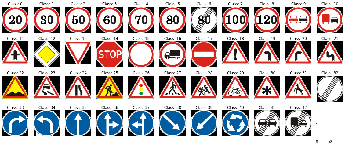
Pictograms of all 43 GTSRB classes, in order. Note that real-world signs may appear in different shapes or colors. See the Visual Key for a full reference to all sign classes.

Some classes are 10× more common than others. Individual classes contain from 150 to 1500 samples, for a total of 26640 images.

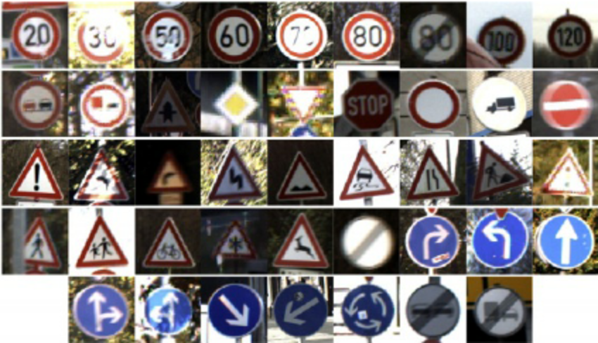
A real-world example of each class, in order, taken directly from the GTSRB dataset. Signs may differ slightly in color, shape, or condition from their pictorial counterparts. See the Visual Key for a full reference to all sign classes.

Model Architecture

Back to Top

Models were developed sequentially, beginning with a baseline and progressively adding complexity. Key modifications included: class weighting to mitigate imbalance; additional convolutional layers for richer feature extraction; batch normalization to stabilize training and improve calibration; and additional dense layers, which in practice reduced performance.

The seven models implemented were:

1. Baseline Model
2. Baseline Model + Class Weights
3. Baseline Model + Second Conv Layer
4. Baseline Model + Batch Normalization
5. Baseline Model + Second Conv Layer + Batch Normalization (best performing)
6. Baseline Model + Second Conv Layer + Dense Layer
7. Baseline Model + Second Conv Layer + Dense Layer + Batch Normalization

Each component played a distinct role in shaping performance. Convolutional layers expanded the network’s ability to capture complex visual patterns, while batch normalization reduced internal variance, improving stability and generalization. Class weighting helped protect minority classes from being overshadowed by frequent categories. Dense layers, while theoretically enabling deeper decision boundaries, tended to disrupt calibration and reduce confidence when convolutional features were already strong.

All models were trained on the GTSRB training set and evaluated on a held-out validation/test split. Inputs were resized to 30×30, balancing detail with efficiency. Training used categorical cross-entropy loss with the Adam optimizer and early stopping to prevent overfitting. Accuracy served as the primary benchmark, supplemented by class-level precision, recall, and F1-scores to capture performance across all 43 categories.

Training and Evaluation Results

Back to Top

The following outputs summarize training and evaluation results for each model:

Model Summary

• Each evaluation begins with a brief recap of the model’s architecture, highlighting which modifications are active.

Training and Loss Curves

• Accuracy and loss curves track learning over time. With Dropout active, validation metrics may surpass training. Smooth convergence suggests stable learning; divergence signals overfitting or regularization effects.

Confusion Matrix

• Confusion matrices plot predicted vs. true labels across all 43 classes. Most cells are empty; performance is judged by the sharpness of the diagonal. Off-diagonal errors highlight confusion among visually similar categories, especially within the upper-left speed-limit cluster.

Classification Report

• Reports show precision, recall, F1-score, and support for each class. Comparing majority vs. minority categories reveals whether rare signs are recognized reliably or collapse into false negatives. Weighted averages summarize overall performance.

Error & Misclassification Analysis

• Grids of the most frequent misclassifications display the true label, predicted label, and model confidence. Any blurriness reflects convolutional feature extraction, not dataset quality. A text summary reports total misclassifications and the top error types (commonly confusion between similar speed limits). A histogram of misclassification confidence distinguishes uncertain errors from systematic blind spots.

Together, these outputs provide a detailed view of each model’s behavior, setting the stage for cross-model comparison.

Baseline Model

Back to Top

The baseline follows a classic MNIST-style CNN: one convolutional layer (32 filters, 3×3, ReLU), max pooling, flattening, a dense layer of 128 units with dropout (0.5), and a softmax output.

Classification Report

	precision	recall	f1-score	support
accuracy	0.965653	0.965653	0.965653	0.965653
macro avg	0.967660	0.955663	0.960694	5328.000000
weighted avg	0.967178	0.965653	0.965741	5328.000000
0	1.000000	0.843750	0.915254	32.000000
1	0.945017	0.961538	0.953206	286.000000
2	0.967033	0.897959	0.931217	294.000000
3	0.955752	0.919149	0.937093	235.000000
4	0.963370	0.981343	0.972274	268.000000
5	0.817844	0.964912	0.885312	228.000000
6	0.981481	0.981481	0.981481	54.000000
7	0.976744	0.918033	0.946479	183.000000
8	0.965174	0.960396	0.962779	202.000000
9	0.989848	0.989848	0.989848	197.000000
10	0.988372	0.980769	0.984556	260.000000
11	0.960894	0.955556	0.958217	180.000000
12	0.993031	1.000000	0.996503	285.000000
13	0.993355	1.000000	0.996667	299.000000
14	1.000000	0.990291	0.995122	103.000000
15	1.000000	0.988764	0.994350	89.000000
16	1.000000	1.000000	1.000000	48.000000
17	0.988889	1.000000	0.994413	178.000000
18	0.959770	0.976608	0.968116	171.000000
19	0.962963	0.838710	0.896552	31.000000
20	0.839286	0.979167	0.903846	48.000000
21	0.977273	0.977273	0.977273	44.000000
22	0.982456	0.949153	0.965517	59.000000
23	0.946667	0.959459	0.953020	74.000000
24	0.973684	0.880952	0.925000	42.000000
25	0.957944	0.995146	0.976190	206.000000
26	0.941860	0.964286	0.952941	84.000000
27	0.914286	0.941176	0.927536	34.000000
28	1.000000	0.923077	0.960000	65.000000
29	0.966667	0.852941	0.906250	34.000000
30	0.981481	0.841270	0.905983	63.000000
31	0.972477	0.990654	0.981481	107.000000
32	0.942857	0.916667	0.929577	36.000000
33	1.000000	0.988636	0.994286	88.000000
34	1.000000	0.936170	0.967033	47.000000
35	1.000000	0.980769	0.990291	156.000000
36	0.918919	0.971429	0.944444	35.000000
37	1.000000	1.000000	1.000000	17.000000
38	0.986667	1.000000	0.993289	296.000000
39	1.000000	1.000000	1.000000	49.000000
40	0.977273	0.977273	0.977273	44.000000
41	0.944444	0.918919	0.931507	37.000000
42	0.975610	1.000000	0.987654	40.000000

Total Misclassifications: 183

Top 5 Most Common Misclassifications:

* Speed limit (50km/h) (label 2) predicted as Speed limit (80km/h) (label 5) — 18 times

* Speed limit (60km/h) (label 3) predicted as Speed limit (80km/h) (label 5) — 14 times

* Speed limit (100km/h) (label 7) predicted as Speed limit (80km/h) (label 5) — 11 times

* Speed limit (50km/h) (label 2) predicted as Speed limit (30km/h) (label 1) — 5 times

* Speed limit (30km/h) (label 1) predicted as Speed limit (50km/h) (label 2) — 5 times

Results for Baseline Model

The model achieves 96.6% accuracy, with weighted precision/recall/F1 around 0.96–0.97. Most classes exceed 0.95, but confusion among visually similar speed-limit signs (class 5, precision 0.82) and several mid-sized classes (e.g., class 20 precision 0.84, class 30 recall 0.84) lowers performance. Minority classes are inconsistent: some perfect, others lagging (e.g., class 19 recall 0.84). Training/validation curves show a small dropout-induced gap, no sign of overfitting. Calibration appears smooth.

Interpretation

A solid baseline with strong overall performance but clear weaknesses in imbalanced and visually similar categories.

Baseline Model with Class Weights

Back to Top

Architecture is unchanged; class weights were applied to address imbalance.

Classification Report

	precision	recall	f1-score	support
accuracy	0.958333	0.958333	0.958333	0.958333
macro avg	0.967206	0.969188	0.967458	5328.000000
weighted avg	0.960015	0.958333	0.958143	5328.000000
0	1.000000	0.906250	0.950820	32.000000
1	0.935154	0.958042	0.946459	286.000000
2	0.978723	0.782313	0.869565	294.000000
3	0.857692	0.948936	0.901010	235.000000
4	0.953069	0.985075	0.968807	268.000000
5	0.784810	0.815789	0.800000	228.000000
6	0.947368	1.000000	0.972973	54.000000
7	0.940476	0.863388	0.900285	183.000000
8	0.858407	0.960396	0.906542	202.000000
9	0.989744	0.979695	0.984694	197.000000
10	0.996094	0.980769	0.988372	260.000000
11	0.988372	0.944444	0.965909	180.000000
12	0.996503	1.000000	0.998249	285.000000
13	0.993311	0.993311	0.993311	299.000000
14	0.990291	0.990291	0.990291	103.000000
15	0.956989	1.000000	0.978022	89.000000
16	0.979592	1.000000	0.989691	48.000000
17	0.994382	0.994382	0.994382	178.000000
18	0.970930	0.976608	0.973761	171.000000
19	0.937500	0.967742	0.952381	31.000000
20	0.903846	0.979167	0.940000	48.000000
21	1.000000	0.977273	0.988506	44.000000
22	0.966667	0.983051	0.974790	59.000000
23	0.986111	0.959459	0.972603	74.000000
24	1.000000	1.000000	1.000000	42.000000
25	0.980583	0.980583	0.980583	206.000000
26	0.954545	1.000000	0.976744	84.000000
27	0.944444	1.000000	0.971429	34.000000
28	0.969231	0.969231	0.969231	65.000000
29	1.000000	0.882353	0.937500	34.000000
30	0.939394	0.984127	0.961240	63.000000
31	1.000000	0.971963	0.985782	107.000000
32	0.947368	1.000000	0.972973	36.000000
33	0.988764	1.000000	0.994350	88.000000
34	1.000000	1.000000	1.000000	47.000000
35	0.987261	0.993590	0.990415	156.000000
36	0.972222	1.000000	0.985915	35.000000
37	1.000000	1.000000	1.000000	17.000000
38	1.000000	0.996622	0.998308	296.000000
39	1.000000	1.000000	1.000000	49.000000
40	1.000000	0.977273	0.988506	44.000000
41	1.000000	0.972973	0.986301	37.000000
42	1.000000	1.000000	1.000000	40.000000

Total Misclassifications: 222

Top 5 Most Common Misclassifications:

* Speed limit (50km/h) (label 2) predicted as Speed limit (80km/h) (label 5) — 30 times

* Speed limit (80km/h) (label 5) predicted as Speed limit (60km/h) (label 3) — 25 times

* Speed limit (100km/h) (label 7) predicted as Speed limit (120km/h) (label 8) — 18 times

* Speed limit (50km/h) (label 2) predicted as Speed limit (30km/h) (label 1) — 16 times

* Speed limit (50km/h) (label 2) predicted as Speed limit (60km/h) (label 3) — 9 times

Results for Baseline Model with Class Weights

Accuracy drops slightly to 95.8%, with weighted scores near 0.96. Minority classes benefit (e.g., several now achieve perfect scores), but majority classes show tradeoffs: class 2 recall falls to 0.78 while precision remains 0.98. Class 5 remains problematic, with both precision and recall declining. Calibration stays balanced.

Interpretation

Weighting improves rare-class support but reduces consistency and overall accuracy, highlighting tradeoffs in handling imbalance.

Two Convolutional Layers

Back to Top

Adds a second convolutional layer (64 filters, 3×3, ReLU) to the baseline, after the first conv+pool block.

Classification Report

	precision	recall	f1-score	support
accuracy	0.982733	0.982733	0.982733	0.982733
macro avg	0.984688	0.982062	0.983111	5328.000000
weighted avg	0.983218	0.982733	0.982749	5328.000000
0	1.000000	0.968750	0.984127	32.000000
1	0.982517	0.982517	0.982517	286.000000
2	0.992857	0.945578	0.968641	294.000000
3	0.970085	0.965957	0.968017	235.000000
4	0.974170	0.985075	0.979592	268.000000
5	0.895582	0.978070	0.935010	228.000000
6	1.000000	0.981481	0.990654	54.000000
7	0.976608	0.912568	0.943503	183.000000
8	0.961353	0.985149	0.973105	202.000000
9	0.989848	0.989848	0.989848	197.000000
10	1.000000	0.988462	0.994197	260.000000
11	1.000000	0.966667	0.983051	180.000000
12	0.996503	1.000000	0.998249	285.000000
13	0.990066	1.000000	0.995008	299.000000
14	1.000000	0.990291	0.995122	103.000000
15	0.956989	1.000000	0.978022	89.000000
16	1.000000	1.000000	1.000000	48.000000
17	0.994413	1.000000	0.997199	178.000000
18	0.982456	0.982456	0.982456	171.000000
19	1.000000	0.935484	0.966667	31.000000
20	1.000000	0.979167	0.989474	48.000000
21	0.956522	1.000000	0.977778	44.000000
22	1.000000	1.000000	1.000000	59.000000
23	1.000000	0.972973	0.986301	74.000000
24	0.954545	1.000000	0.976744	42.000000
25	0.980952	1.000000	0.990385	206.000000
26	0.964706	0.976190	0.970414	84.000000
27	0.944444	1.000000	0.971429	34.000000
28	1.000000	1.000000	1.000000	65.000000
29	1.000000	0.911765	0.953846	34.000000
30	0.984127	0.984127	0.984127	63.000000
31	0.990654	0.990654	0.990654	107.000000
32	0.941176	0.888889	0.914286	36.000000
33	0.988764	1.000000	0.994350	88.000000
34	1.000000	1.000000	1.000000	47.000000
35	1.000000	0.993590	0.996785	156.000000
36	0.972222	1.000000	0.985915	35.000000
37	1.000000	1.000000	1.000000	17.000000
38	1.000000	1.000000	1.000000	296.000000
39	1.000000	1.000000	1.000000	49.000000
40	1.000000	1.000000	1.000000	44.000000
41	1.000000	0.972973	0.986301	37.000000
42	1.000000	1.000000	1.000000	40.000000

Total Misclassifications: 92

Top 5 Most Common Misclassifications:

* Speed limit (50km/h) (label 2) predicted as Speed limit (80km/h) (label 5) — 11 times

* Speed limit (60km/h) (label 3) predicted as Speed limit (80km/h) (label 5) — 7 times

* Speed limit (100km/h) (label 7) predicted as Speed limit (120km/h) (label 8) — 6 times

* Speed limit (100km/h) (label 7) predicted as Speed limit (80km/h) (label 5) — 6 times

* Speed limit (30km/h) (label 1) predicted as Speed limit (70km/h) (label 4) — 4 times

Results for Two Convolutional Layers

Accuracy rises to 98.3%, with weighted scores ~0.98. Class 5 improves markedly (precision 0.90, recall 0.98), and most historically weak classes achieve >0.95. Nearly all minority classes reach perfect performance, with only a few lagging slightly (e.g., class 32 F1 = 0.91). Training and validation curves are tightly matched. No overfitting is observed.

Interpretation

Deeper convolution improves feature extraction and generalization, outperforming both baseline and weighted models across nearly all classes.

Baseline Model with Batch Normalization

Back to Top

Adding batch normalization after the first convolution stabilizes training and accelerates convergence. The rest of the architecture mirrors the baseline.

Classification Report

	precision	recall	f1-score	support
accuracy	0.982545	0.982545	0.982545	0.982545
macro avg	0.986344	0.978723	0.982302	5328.000000
weighted avg	0.982805	0.982545	0.982484	5328.000000
0	0.939394	0.968750	0.953846	32.000000
1	0.952703	0.986014	0.969072	286.000000
2	0.956954	0.982993	0.969799	294.000000
3	0.990741	0.910638	0.949002	235.000000
4	0.974265	0.988806	0.981481	268.000000
5	0.952586	0.969298	0.960870	228.000000
6	1.000000	1.000000	1.000000	54.000000
7	0.971910	0.945355	0.958449	183.000000
8	0.985000	0.975248	0.980100	202.000000
9	1.000000	0.994924	0.997455	197.000000
10	1.000000	0.992308	0.996139	260.000000
11	0.951872	0.988889	0.970027	180.000000
12	0.993031	1.000000	0.996503	285.000000
13	0.990066	1.000000	0.995008	299.000000
14	1.000000	1.000000	1.000000	103.000000
15	0.988889	1.000000	0.994413	89.000000
16	1.000000	1.000000	1.000000	48.000000
17	1.000000	0.994382	0.997183	178.000000
18	0.982558	0.988304	0.985423	171.000000
19	0.967742	0.967742	0.967742	31.000000
20	1.000000	0.958333	0.978723	48.000000
21	1.000000	0.977273	0.988506	44.000000
22	0.966667	0.983051	0.974790	59.000000
23	0.986301	0.972973	0.979592	74.000000
24	0.975610	0.952381	0.963855	42.000000
25	0.962617	1.000000	0.980952	206.000000
26	0.976471	0.988095	0.982249	84.000000
27	1.000000	0.970588	0.985075	34.000000
28	0.984127	0.953846	0.968750	65.000000
29	0.966667	0.852941	0.906250	34.000000
30	1.000000	0.968254	0.983871	63.000000
31	1.000000	1.000000	1.000000	107.000000
32	1.000000	0.972222	0.985915	36.000000
33	1.000000	1.000000	1.000000	88.000000
34	1.000000	1.000000	1.000000	47.000000
35	1.000000	0.993590	0.996785	156.000000
36	1.000000	0.971429	0.985507	35.000000
37	1.000000	1.000000	1.000000	17.000000
38	0.996610	0.993243	0.994924	296.000000
39	1.000000	1.000000	1.000000	49.000000
40	1.000000	0.977273	0.988506	44.000000
41	1.000000	0.945946	0.972222	37.000000
42	1.000000	1.000000	1.000000	40.000000

Total Misclassifications: 93

Top 5 Most Common Misclassifications:

* Speed limit (60km/h) (label 3) predicted as Speed limit (50km/h) (label 2) — 6 times

* Speed limit (100km/h) (label 7) predicted as Speed limit (80km/h) (label 5) — 5 times

* Speed limit (50km/h) (label 2) predicted as Speed limit (30km/h) (label 1) — 4 times

* Speed limit (60km/h) (label 3) predicted as Speed limit (80km/h) (label 5) — 4 times

* Speed limit (60km/h) (label 3) predicted as Speed limit (30km/h) (label 1) — 3 times

Results for Baseline Model with Batch Normalization

Accuracy improves to 98.3% (precision/recall/f1 ≈ 0.983), outperforming both the plain baseline (96.6%) and class-weighted variant (95.8%). Class 5 in particular improves sharply (f1 = 0.96 vs. 0.80–0.88 before). Minority classes remain strong, with many perfect scores. Training and validation curves track together. Confidence scores cluster higher without harming calibration.

Interpretation

Batch normalization is as effective as adding depth for boosting performance, while also providing smoother training dynamics and stability. It resolves weaknesses in confusing classes like 5 without sacrificing generalization.

Two Convolutional Layers with Batch Normalization

Back to Top

This design stacks two convolutional layers, each followed by batch normalization and pooling, before dense/dropout and softmax.

Classification Report

	precision	recall	f1-score	support
accuracy	0.994182	0.994182	0.994182	0.994182
macro avg	0.995007	0.993229	0.994045	5328.000000
weighted avg	0.994251	0.994182	0.994180	5328.000000
0	1.000000	0.968750	0.984127	32.000000
1	0.993056	1.000000	0.996516	286.000000
2	0.993151	0.986395	0.989761	294.000000
3	0.991561	1.000000	0.995763	235.000000
4	0.992565	0.996269	0.994413	268.000000
5	0.969957	0.991228	0.980477	228.000000
6	1.000000	0.981481	0.990654	54.000000
7	0.977901	0.967213	0.972527	183.000000
8	0.994949	0.975248	0.985000	202.000000
9	1.000000	0.989848	0.994898	197.000000
10	1.000000	0.996154	0.998073	260.000000
11	1.000000	0.994444	0.997214	180.000000
12	0.996503	1.000000	0.998249	285.000000
13	0.996667	1.000000	0.998331	299.000000
14	1.000000	1.000000	1.000000	103.000000
15	1.000000	0.988764	0.994350	89.000000
16	1.000000	1.000000	1.000000	48.000000
17	1.000000	1.000000	1.000000	178.000000
18	1.000000	1.000000	1.000000	171.000000
19	1.000000	1.000000	1.000000	31.000000
20	0.960000	1.000000	0.979592	48.000000
21	1.000000	1.000000	1.000000	44.000000
22	1.000000	1.000000	1.000000	59.000000
23	1.000000	0.986486	0.993197	74.000000
24	1.000000	1.000000	1.000000	42.000000
25	0.980861	0.995146	0.987952	206.000000
26	1.000000	1.000000	1.000000	84.000000
27	1.000000	1.000000	1.000000	34.000000
28	1.000000	1.000000	1.000000	65.000000
29	1.000000	0.941176	0.969697	34.000000
30	1.000000	1.000000	1.000000	63.000000
31	0.990741	1.000000	0.995349	107.000000
32	0.947368	1.000000	0.972973	36.000000
33	1.000000	1.000000	1.000000	88.000000
34	1.000000	1.000000	1.000000	47.000000
35	1.000000	1.000000	1.000000	156.000000
36	1.000000	1.000000	1.000000	35.000000
37	1.000000	1.000000	1.000000	17.000000
38	1.000000	1.000000	1.000000	296.000000
39	1.000000	1.000000	1.000000	49.000000
40	1.000000	0.977273	0.988506	44.000000
41	1.000000	0.972973	0.986301	37.000000
42	1.000000	1.000000	1.000000	40.000000

Total Misclassifications: 31

Top 5 Most Common Misclassifications:

* Speed limit (120km/h) (label 8) predicted as Speed limit (100km/h) (label 7) — 4 times

* Speed limit (50km/h) (label 2) predicted as Speed limit (80km/h) (label 5) — 3 times

* Speed limit (100km/h) (label 7) predicted as Speed limit (80km/h) (label 5) — 3 times

* Road work (label 25) predicted as Dangerous curve to the right (label 20) — 1 times

* End of no passing (label 41) predicted as End of all speed and passing limits (label 32) — 1 times

Results for Two Convolutional Layers with Batch Normalization

This model achieves the best results overall: 99.4% accuracy with precision/recall/f1 ≈ 0.994. Nearly all classes are perfectly classified, including those that previously lagged (e.g., class 5 with f1 = 0.98). Training and validation curves are tightly matched. Predictions are both accurate and highly confident, with almost no systematic errors.

Interpretation

Combining depth with batch normalization sets the benchmark, delivering near-perfect results across the board. It maximizes both accuracy and stability, leaving little room for improvement.

Two Convolutional + Dense Layers

Back to Top

This variant extends the two-conv backbone with a second dense layer after flattening.

Classification Report

	precision	recall	f1-score	support
accuracy	0.938251	0.938251	0.938251	0.938251
macro avg	0.915974	0.885795	0.890472	5328.000000
weighted avg	0.937184	0.938251	0.932645	5328.000000
0	1.000000	0.781250	0.877193	32.000000
1	0.961938	0.972028	0.966957	286.000000
2	0.979522	0.976190	0.977853	294.000000
3	0.982222	0.940426	0.960870	235.000000
4	0.963504	0.985075	0.974170	268.000000
5	0.898374	0.969298	0.932489	228.000000
6	0.980392	0.925926	0.952381	54.000000
7	1.000000	0.655738	0.792079	183.000000
8	0.764228	0.930693	0.839286	202.000000
9	0.989848	0.989848	0.989848	197.000000
10	0.977273	0.992308	0.984733	260.000000
11	0.857868	0.938889	0.896552	180.000000
12	0.982759	1.000000	0.991304	285.000000
13	0.980328	1.000000	0.990066	299.000000
14	1.000000	0.980583	0.990196	103.000000
15	0.956989	1.000000	0.978022	89.000000
16	0.979592	1.000000	0.989691	48.000000
17	0.983425	1.000000	0.991643	178.000000
18	0.888889	0.982456	0.933333	171.000000
19	1.000000	0.870968	0.931034	31.000000
20	0.969697	0.666667	0.790123	48.000000
21	0.977273	0.977273	0.977273	44.000000
22	1.000000	0.983051	0.991453	59.000000
23	0.829545	0.986486	0.901235	74.000000
24	0.000000	0.000000	0.000000	42.000000
25	0.962441	0.995146	0.978520	206.000000
26	0.653061	0.761905	0.703297	84.000000
27	0.875000	0.205882	0.333333	34.000000
28	0.563636	0.953846	0.708571	65.000000
29	0.961538	0.735294	0.833333	34.000000
30	0.828571	0.460317	0.591837	63.000000
31	0.963303	0.981308	0.972222	107.000000
32	0.868421	0.916667	0.891892	36.000000
33	0.988764	1.000000	0.994350	88.000000
34	1.000000	0.936170	0.967033	47.000000
35	0.993631	1.000000	0.996805	156.000000
36	1.000000	0.857143	0.923077	35.000000
37	0.894737	1.000000	0.944444	17.000000
38	0.973684	1.000000	0.986667	296.000000
39	0.979167	0.959184	0.969072	49.000000
40	0.977273	0.977273	0.977273	44.000000
41	1.000000	0.918919	0.957746	37.000000
42	1.000000	0.925000	0.961039	40.000000

Total Misclassifications: 329

Top 5 Most Common Misclassifications:

* Speed limit (100km/h) (label 7) predicted as Speed limit (120km/h) (label 8) — 51 times

* Road narrows on the right (label 24) predicted as Children crossing (label 28) — 38 times

* Beware of ice/snow (label 30) predicted as Right-of-way at the next intersection (label 11) — 28 times

* Pedestrians (label 27) predicted as Traffic signals (label 26) — 26 times

* Traffic signals (label 26) predicted as General caution (label 18) — 20 times

Results for Two Convolutional + Dense Layers

Performance drops sharply to 93.8% accuracy (precision/recall/f1 ≈ 0.93). Several classes collapse completely (e.g., class 24, f1 = 0.0), and many mid-frequency categories degrade. A large gap with validation outperforming training—especially with Dropout—indicates strong regularization. The model is less confident and less accurate overall, with poor calibration and weak generalization.

Interpretation

Adding complexity at the dense stage destabilizes training and impairs calibration. Rather than capturing richer patterns, the extra dense layer disrupts feature extraction, leading to lower confidence, unreliable predictions, and poor generalization.

Two Convolutional + Dense Layers with Batch Normalization

Back to Top

This model applies batch normalization to the two-conv/two-dense architecture.

Classification Report

	precision	recall	f1-score	support
accuracy	0.983108	0.983108	0.983108	0.983108
macro avg	0.981243	0.975459	0.976832	5328.000000
weighted avg	0.983436	0.983108	0.982712	5328.000000
0	0.944444	0.531250	0.680000	32.000000
1	0.943709	0.996503	0.969388	286.000000
2	0.996503	0.969388	0.982759	294.000000
3	0.986900	0.961702	0.974138	235.000000
4	1.000000	0.996269	0.998131	268.000000
5	0.945148	0.982456	0.963441	228.000000
6	1.000000	1.000000	1.000000	54.000000
7	0.964072	0.879781	0.920000	183.000000
8	0.903226	0.970297	0.935561	202.000000
9	0.994924	0.994924	0.994924	197.000000
10	0.996154	0.996154	0.996154	260.000000
11	1.000000	0.983333	0.991597	180.000000
12	1.000000	1.000000	1.000000	285.000000
13	0.996667	1.000000	0.998331	299.000000
14	0.990291	0.990291	0.990291	103.000000
15	0.988889	1.000000	0.994413	89.000000
16	0.979592	1.000000	0.989691	48.000000
17	0.994413	1.000000	0.997199	178.000000
18	0.994186	1.000000	0.997085	171.000000
19	0.935484	0.935484	0.935484	31.000000
20	0.958333	0.958333	0.958333	48.000000
21	1.000000	1.000000	1.000000	44.000000
22	1.000000	1.000000	1.000000	59.000000
23	1.000000	0.972973	0.986301	74.000000
24	0.976744	1.000000	0.988235	42.000000
25	1.000000	0.990291	0.995122	206.000000
26	1.000000	0.988095	0.994012	84.000000
27	0.971429	1.000000	0.985507	34.000000
28	0.970149	1.000000	0.984848	65.000000
29	1.000000	1.000000	1.000000	34.000000
30	0.967742	0.952381	0.960000	63.000000
31	0.963964	1.000000	0.981651	107.000000
32	0.972973	1.000000	0.986301	36.000000
33	1.000000	1.000000	1.000000	88.000000
34	1.000000	1.000000	1.000000	47.000000
35	0.993631	1.000000	0.996805	156.000000
36	0.972222	1.000000	0.985915	35.000000
37	0.944444	1.000000	0.971429	17.000000
38	1.000000	0.996622	0.998308	296.000000
39	1.000000	1.000000	1.000000	49.000000
40	1.000000	0.977273	0.988506	44.000000
41	0.972222	0.945946	0.958904	37.000000
42	0.975000	0.975000	0.975000	40.000000

Total Misclassifications: 90

Top 5 Most Common Misclassifications:

* Speed limit (100km/h) (label 7) predicted as Speed limit (120km/h) (label 8) — 18 times

* Speed limit (20km/h) (label 0) predicted as Speed limit (30km/h) (label 1) — 15 times

* Speed limit (50km/h) (label 2) predicted as Speed limit (80km/h) (label 5) — 5 times

* Speed limit (60km/h) (label 3) predicted as Speed limit (80km/h) (label 5) — 5 times

* Speed limit (120km/h) (label 8) predicted as Speed limit (100km/h) (label 7) — 4 times

Results for Two Convolutional + Dense Layers, and Batch Normalization

Accuracy recovers somewhat to 98.3% (precision/recall/f1 ≈ 0.983) but remains below the simpler two-conv + batch norm design. Most classes perform well, but consistency suffers: e.g., class 0 recall drops to 0.53. The added dense layer complicates decision boundaries without real gain.

Interpretation

Batch normalization restores stability but cannot offset the drawbacks of extra dense complexity. While accurate overall, the model introduces instability in key classes, showing that simplicity with batch normalization remains the optimal choice.

Model Comparison and Analysis

Back to Top

Model progression shows how each architectural tweak affects performance. The best model balances depth and stability—more convolution and normalization help, while extra dense layers only hinder.

Model Comparison Table

Model	Accuracy	Precision	Recall	F1-score	Errors	Notes
Baseline Model	96.6%	0.967	0.966	0.966	183	Solid foundation; struggles with minority classes.
+ Class Weights	95.8%	0.960	0.958	0.958	222	Improves minority class metrics; reduces majority performance. Tradeoff observed.
+ Conv Layer	98.3%	0.983	0.983	0.983	92	Enhanced feature extraction; reduces confusion among similar signs.
+ Batch Norm	98.3%	0.983	0.983	0.982	93	Stabilizes training and accelerates convergence; yields more consistent results.
+ Conv + BN	99.4%	0.994	0.994	0.994	31	Strongest overall—high accuracy, few errors across classes.
+ Conv + Dense	93.8%	0.937	0.938	0.933	329	Added complexity degrades performance; some classes collapse.
+ Conv + Dense + BN	98.3%	0.983	0.983	0.983	90	No improvement over Conv+BN; simpler architecture prevails.

Accuracy: Proportion of all predictions that are correct.
Precision: Proportion of positive predictions that are correct (True Positives / [True Positives + False Positives]).
Recall: Proportion of actual positives correctly identified (True Positives / [True Positives + False Negatives]).
F1-score: Harmonic mean balancing precision and recall equally.
Errors: Number of misclassifications of 5,328 total samples in validation set.

Baseline Model

A simple MNIST-style CNN achieved 96.6% accuracy with strong class-level balance, but struggled with visually similar signs (e.g., speed limits) and some minority categories. Solid foundation but systematic challenges remain.

+Class Weights

Minority classes (e.g., 19, 29) improved in recall and precision, but majority classes lost ground, dropping overall accuracy to 95.8%. Highlights the inherent tradeoff in rebalancing imbalanced datasets.

+Convolutional Layer

Adding a second conv layer boosted accuracy to 98.3% by extracting richer features, reducing confusion among similar signs, and stabilizing minority performance. Clear gain without overfitting.

+Batch Normalization

Batch normalization maintained 98.3% accuracy but smoothed training and improved calibration, especially for minority classes. Reduced variance across runs, yielding more reliable results.

+Convolutional Layer + Batch Normalization

The optimal model: 99.4% accuracy, balanced across nearly all classes, with previously weak categories (e.g., class 5) substantially improved. Depth plus normalization proved the strongest combination.

+Dense Layer

Adding an extra dense layer destabilized training, collapsing several classes and cutting accuracy to 93.8%. Demonstrates the risk of unnecessary complexity.

+Dense Layer + Batch Normalization

Batch normalization partially mitigated dense-layer instability, recovering to 98.3%. Still fell short of Conv+BN, confirming that added dense layers do not improve generalization.

Overall Trajectory

Accuracy improved from 96.6% (Baseline) to 99.4% (+Conv+BN). Class weighting improved minorities but weakened majority performance; convolutional depth enhanced feature extraction; batch normalization stabilized training and calibration. Extra dense layers consistently underperformed. The two-convolutional-layer + BN model struck the best balance of accuracy, stability, and class-level consistency.

And the winner is...

Two Convolutional Layers with Batch Normalization

This model achieved 99.4% validation accuracy with balanced precision/recall and minimal error.

Final Test Set Evaluation

Back to Top

With training done, the real test is unseen data. The top model—two convolutional layers plus batch normalization—was evaluated on the GTSRB test set. Results confirm strong generalization, balanced class performance, and robust handling of real-world conditions.

Classification Report

	precision	recall	f1-score	support
accuracy	0.991929	0.991929	0.991929	0.991929
macro avg	0.990396	0.991160	0.990690	5328.000000
weighted avg	0.991979	0.991929	0.991921	5328.000000
0	0.961538	0.961538	0.961538	26.000000
1	0.989761	0.989761	0.989761	293.000000
2	0.990260	0.983871	0.987055	310.000000
3	0.979275	0.994737	0.986945	190.000000
4	0.992453	0.988722	0.990584	266.000000
5	0.976285	0.968627	0.972441	255.000000
6	0.985075	1.000000	0.992481	66.000000
7	1.000000	0.983607	0.991736	183.000000
8	0.988827	1.000000	0.994382	177.000000
9	1.000000	0.995169	0.997579	207.000000
10	0.996503	1.000000	0.998249	285.000000
11	1.000000	0.995074	0.997531	203.000000
12	0.996310	1.000000	0.998152	270.000000
13	1.000000	1.000000	1.000000	281.000000
14	1.000000	1.000000	1.000000	93.000000
15	1.000000	1.000000	1.000000	83.000000
16	1.000000	1.000000	1.000000	72.000000
17	0.992647	1.000000	0.996310	135.000000
18	0.987730	1.000000	0.993827	161.000000
19	0.958333	1.000000	0.978723	23.000000
20	1.000000	0.978723	0.989247	47.000000
21	1.000000	0.975610	0.987654	41.000000
22	1.000000	1.000000	1.000000	46.000000
23	0.987342	1.000000	0.993631	78.000000
24	0.945946	1.000000	0.972222	35.000000
25	0.989691	0.989691	0.989691	194.000000
26	0.987342	1.000000	0.993631	78.000000
27	1.000000	0.944444	0.971429	36.000000
28	1.000000	1.000000	1.000000	72.000000
29	1.000000	0.945946	0.972222	37.000000
30	1.000000	1.000000	1.000000	56.000000
31	0.976000	0.968254	0.972112	126.000000
32	1.000000	1.000000	1.000000	38.000000
33	1.000000	1.000000	1.000000	93.000000
34	0.983333	0.983333	0.983333	60.000000
35	0.994083	0.994083	0.994083	169.000000
36	0.985915	0.985915	0.985915	71.000000
37	0.968750	1.000000	0.984127	31.000000
38	0.996377	0.992780	0.994575	277.000000
39	1.000000	1.000000	1.000000	42.000000
40	0.977273	1.000000	0.988506	43.000000
41	1.000000	1.000000	1.000000	47.000000
42	1.000000	1.000000	1.000000	32.000000

Total Misclassifications: 43

Top 5 Most Common Misclassifications:

* Speed limit (80km/h) (label 5) predicted as Speed limit (60km/h) (label 3) — 4 times

* Speed limit (50km/h) (label 2) predicted as Speed limit (80km/h) (label 5) — 2 times

* Speed limit (100km/h) (label 7) predicted as Speed limit (80km/h) (label 5) — 2 times

* Bicycles crossing (label 29) predicted as Wild animals crossing (label 31) — 2 times

* Speed limit (70km/h) (label 4) predicted as Speed limit (50km/h) (label 2) — 2 times

Results of Test Set Evaluation

On the GTSRB test set, the best model reached 99.2% accuracy, with weighted precision/recall/F1 all at 0.99. Performance was consistent across nearly all classes, with only a few small categories (e.g., 24, 27, 29) dipping slightly (~0.97 F1). Most classes achieved or exceeded 0.99, many at perfection. Misclassifications were rare and mostly involved visually similar speed limit signs.

Interpretation

The final model generalized well, confirming that targeted refinements—extra convolution and batch normalization—drove gains, while unnecessary dense layers hurt stability. Results demonstrate that parsimony outperforms complexity when handling imbalanced, visually similar classes.

Conclusion

Back to Top

From baseline to final, the experiments show that controlled complexity—not sheer size—produces the most effective models. Strategic use of class weighting and normalization closed gaps in minority and confusing classes, yielding a reliable model with near state-of-the-art accuracy.

Future directions could explore higher-resolution inputs, transfer learning, or cross-domain adaptation to further strengthen performance in applied settings.

© 2025 Bryan C. Johns Portfolio LinkedIn GitHub